原文 Hermite Curve Interpolation
Hermite Curve Interpolation
Hamburg (Germany), the 30th March 1998. Written by Nils Pipenbrinck aka Submissive/Cubic & $eeN
Introduction
Hermite curves are very easy to calculate but also very powerful. They are used to smoothly interpolate between key-points (like object movement in keyframe animation or camera control). Understanding the mathematical background of hermite curves will help you to understand the entire family of splines. Maybe you have some experience with 3D programming and have already used them without knowing that (the so called kb-splines, curves with control over tension, continuity and bias are just a special form of the hermite curves).
The Math
To keep it simple we first start with some simple stuff. We also only talk about 2-dimensional curves here. If you need a 3D curve just do with the z-coordinate what you do with y or x. Hermite curves work in in any number of dimensions.
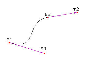
To calculate a hermite curve you need the following vectors:
- P1: the startpoint of the curve
- T1: the tangent (e.g. direction and speed) to how the curve leaves the startpoint
- P2: he endpoint of the curve
- T2: the tangent (e.g. direction and speed) to how the curves meets the endpoint
These 4 vectors are simply multiplied with 4 hermite basis functions and added together.
h1(s) =  2s^3 - 3s^2 + 1
h2(s) = -2s^3 + 3s^2
h3(s) =   s^3 - 2s^2 + s
h4(s) =   s^3 -  s^2
Below are the 4 graphs of the 4 functions (from left to right: h1, h2, h3, h4).
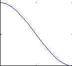
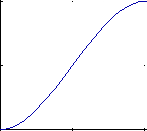
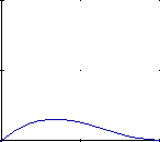
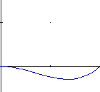
(all graphs except the 4th have been plotted from 0,0 to 1,1)
Take a closer look at functions h1 and h2:
- h1 starts at 1 and goes slowly to 0.
- h2 starts at 0 and goes slowly to 1.
Now multiply the startpoint with h1 and the endpoint with h2. Let s go from 0 to 1 to interpolate between start and endpoint. h3 and h4 are applied to the tangents in the same manner. They make sure that the curve bends in the desired direction at the start and endpoint.
The Math in Matrix Form
All this stuff can be expessed with some vector and matrix algebra. I think the matrix-form is much easier to understand.
Vector S: The interpolation-point and it's powers up to 3:
Vector C: The parameters of our hermite curve:
Matrix h: The matrix form of the 4 hermite polynomials:


     | s^3 |            | P1 |             |  2  -2   1   1 |
S =  | s^2 |       C =  | P2 |        h =  | -3   3  -2  -1 |
     | s^1 |            | T1 |             |  0   0   1   0 |
     | 1   |            | T2 |             |  1   0   0   0 |
To calculate a point on the curve you build the Vector S, multiply it with the matrix h and then multiply with C.P = S * h * C
A little side-note: Bezier-Curves
This matrix-form is valid for all cubic polynomial curves. The only thing that changes is the polynomial matrix. For example, if you want to draw a Bezier curve instead of hermites you might use this matrix:
     | -1   3  -3   1 |
b =  |  3  -6   3   0 |
     | -3   3   0   0 |
     |  1   0   0   0 |
I wrote a separate page about bezier curves.
Some Pseudocode
Sure, this C-style pseudo-code won't compile. C doesn't come with a power function, and unless you wrote yourself a vector-class any compiler would generate hundreds of errors and make you feel like an idiot. I think it's better to present this code in a more abstract form.
moveto (P1);                            // move pen to startpoint
for (int t=0; t < steps; t++)
{
  float s = (float)t / (float)steps;    // scale s to go from 0 to 1
  float h1 =  2s^3 - 3s^2 + 1;          // calculate basis function 1
  float h2 = -2s^3 + 3s^2;              // calculate basis function 2
  float h3 =   s^3 - 2*s^2 + s;         // calculate basis function 3
  float h4 =   s^3 -  s^2;              // calculate basis function 4
  vector p = h1*P1 +                    // multiply and sum all funtions
             h2*P2 +                    // together to build the interpolated
             h3*T1 +                    // point along the curve.
             h4*T2;
  lineto (p)                            // draw to calculated point on the curve
}
Getting rid of the Tangents
I know... controlling the tangents is not easy. It's hard to guess what a curve will look like if you have to define it. Also, to make a sharply bending curve you have to drag the tangent-points far away from the curve. I'll now show you how you can turn the hermite curves into cardinal splines.
Cardinal splines
Cardinal splines are just a subset of the hermite curves. They don't need the tangent points because they will be calculated from the control points. We'll lose some of the flexibility of the hermite curves, but as a tradeoff the curves will be much easier to use. The formula for the tangents for cardinal splines is:
Ti = a * ( Pi+1 - Pi-1 )
a is a constant which affects the tightness of the curve. Write yourself a program and play around with it. ( a should be between 0 and 1, but this is not a must).
Catmull-Rom splines
The Catmull-Rom spline is again just a subset of the cardinal splines. You only have to define a as 0.5, and you can draw and interpolate Catmull-Rom splines.
Ti = 0.5 * ( P i+1 - Pi-1 )
Easy, isn't it? Take a math-book and look for Catmull-Rom splines. Try to understand how they work! It's damn difficult, but when they are derived from hermite curves the cardinal splines turn out to be very easy to understand. Catmull-Rom splines are great if you have some data-points and just want to interpolate smoothly between them.
The Kochanek-Bartels Splines (also called TCB-Splines)
Now we're going down to the guts of curve interpolation. The kb-splines (mostly known from Autodesk's 3d-Studio Max and Newtek's Lightwave) are nothing more than hermite curves and a handfull of formulas to calculate the tangents. These curves have been introduced by D. Kochanek and R. Bartels in 1984 to give animators more control over keyframe animation. They introduced three control-values for each keyframe point:
- Tension: How sharply does the curve bend?
- Continuity: How rapid is the change in speed and direction?
- Bias: What is the direction of the curve as it passes through the keypoint?
I won't try to derive the tangent-formulas here. I think just giving you something you can use is a better idea. (if you're interested you can ask me. I can write it down and send it to you via email.)
The "incoming" Tangent equation:

          (1-t)*(1-c)*(1+b)
TS    =   -----------------  * ( P   -  P    )
  i              2                i      i-1

          (1-t)*(1+c)*(1-b)
      +   -----------------  * ( P   -  P    )
                 2                i+1    i

The "outgoing" Tangent equation:

          (1-t)*(1+c)*(1+b)
TD    =   -----------------  * ( P   -  P    )
  i              2                i      i-1

          (1-t)*(1-c)*(1-b)
      +   -----------------  * ( P   -  P    )
                 2                i+1    i

When you want to interpolate the curve you should use this vector:

    |  P(i)    |
C = |  P(i+1)  |
    |  TD(i)   |
    |  TS(i+1) |
You might notice that you always need the previous and next point if you want to calculate the curve. This might be a problem when you try to calculate keyframe data from Lightwave or 3D-Studio. I don't know exactly how these programs handle the cases of the first and last point, but there are enough sources available on the internet. Just search around a little bit. (Newtek has a good developer section. You can download the origignal Lightwave motion code on their web-site).
Speed Control
If you write yourself keyframe-interpolation code and put it into a program you'll notice one problem. Unless you have your keyframes in fixed intervals you will have a sudden change of speed and direction whenever you pass a keyframe-point. This can be avoided if you take the number of key-positions (frames) between two keyframes into account:
N is the number of frames (seconds, whatever) between two keypoints.

                    2 * N
                         i-1
TD  =  TD *     ---------------       adjustment of outgoing tangent
  i      i          N    + N
                     i-1    i


                    2 * N
                         i
TS  =  TS *     ---------------       adjustment of incomming tangent
  i      i          N    + N
                     i-1    i
What about the "normal" Splines?
The other spline-types, beta-splines, uniform nonrational splines and all the others are a completely different thing and are not covered here. They share one thing with the hermite curves: They are still cubic polynomials, but the way they are calculated is different.
Final Words
Why does no-one care that it's almost impossible to do nicely formatted math-formulas in HTML? What's more important? Good design or good content? As always you might want to contact me.