A Gentle Introduction to the Gradient Boosting Algorithm for Machine Learning
Gradient boosting is one of the most powerful techniques for building predictive models.
In this post you will discover the gradient boosting machine learning algorithm and get a gentle introduction into where it came from and how it works.
After reading this post, you will know:
- The origin of boosting from learning theory and AdaBoost.
- How gradient boosting works including the loss function, weak learners and the additive model.
- How to improve performance over the base algorithm with various regularization schemes
Let’s get started.

A Gentle Introduction to the Gradient Boosting Algorithm for Machine Learning
Photo by brando.n, some rights reserved.
The Algorithm that is Winning Competitions
...XGBoost for fast gradient boosting
 XGBoost is the high performance implementation of gradient boosting that you can now access directly in Python.
Your PDF Download and Email Course.
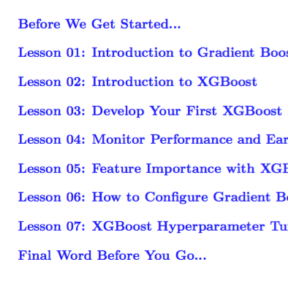
FREE 7-Day Mini-Course on
XGBoost With Python
Download Your FREE Mini-Course
Download your PDF containing all 7 lessons.
Daily lesson via email with tips and tricks.
The Origin of Boosting
The idea of boosting came out of the idea of whether a weak learner can be modified to become better.
Michael Kearns articulated the goal as the “Hypothesis Boosting Problem” stating the goal from a practical standpoint as:
… an efficient algorithm for converting relatively poor hypotheses into very good hypotheses
— Thoughts on Hypothesis Boosting [PDF], 1988
A weak hypothesis or weak learner is defined as one whose performance is at least slightly better than random chance.
These ideas built upon Leslie Valiant’s work on distribution free or Probability Approximately Correct (PAC) learning, a framework for investigating the complexity of machine learning problems.
Hypothesis boosting was the idea of filtering observations, leaving those observations that the weak learner can handle and focusing on developing new weak learns to handle the remaining difficult observations.
The idea is to used the weak learning method several times to get a succession of hypotheses, each one refocused on the examples that the previous ones found difficult and misclassified. … Note, however, it is not obvious at all how this can be done
— Probably Approximately Correct: Nature’s Algorithms for Learning and Prospering in a Complex World, page 152, 2013
AdaBoost the First Boosting Algorithm
The first realization of boosting that saw great success in application was Adaptive Boosting or AdaBoost for short.
Boosting refers to this general problem of producing a very accurate prediction rule by combining rough and moderately inaccurate rules-of-thumb.
— A decision-theoretic generalization of on-line learning and an application to boosting [PDF], 1995
The weak learners in AdaBoost are decision trees with a single split, called decision stumps for their shortness.
AdaBoost works by weighting the observations, putting more weight on difficult to classify instances and less on those already handled well. New weak learners are added sequentially that focus their training on the more difficult patterns.
This means that samples that are difficult to classify receive increasing larger weights until the algorithm identifies a model that correctly classifies these samples
— Applied Predictive Modeling, 2013
Predictions are made by majority vote of the weak learners’ predictions, weighted by their individual accuracy. The most successful form of the AdaBoost algorithm was for binary classification problems and was called AdaBoost.M1.
You can learn more about the AdaBoost algorithm in the post:
Generalization of AdaBoost as Gradient Boosting
AdaBoost and related algorithms were recast in a statistical framework first by Breiman calling them ARCing algorithms.
Arcing is an acronym for Adaptive Reweighting and Combining. Each step in an arcing algorithm consists of a weighted minimization followed by a recomputation of [the classifiers] and [weighted input].
— Prediction Games and Arching Algorithms [PDF], 1997
This framework was further developed by Friedman and called Gradient Boosting Machines. Later called just gradient boosting or gradient tree boosting.
The statistical framework cast boosting as a numerical optimization problem where the objective is to minimize the loss of the model by adding weak learners using a gradient descent like procedure.
This class of algorithms were described as a stage-wise additive model. This is because one new weak learner is added at a time and existing weak learners in the model are frozen and left unchanged.
Note that this stagewise strategy is different from stepwise approaches that readjust previously entered terms when new ones are added.
— Greedy Function Approximation: A Gradient Boosting Machine [PDF], 1999
The generalization allowed arbitrary differentiable loss functions to be used, expanding the technique beyond binary classification problems to support regression, multi-class classification and more.
How Gradient Boosting Works
Gradient boosting involves three elements:
- A loss function to be optimized.
- A weak learner to make predictions.
- An additive model to add weak learners to minimize the loss function.
1. Loss Function
The loss function used depends on the type of problem being solved.
It must be differentiable, but many standard loss functions are supported and you can define your own.
For example, regression may use a squared error and classification may use logarithmic loss.
A benefit of the gradient boosting framework is that a new boosting algorithm does not have to be derived for each loss function that may want to be used, instead, it is a generic enough framework that any differentiable loss function can be used.
2. Weak Learner
Decision trees are used as the weak learner in gradient boosting.
Specifically regression trees are used that output real values for splits and whose output can be added together, allowing subsequent models outputs to be added and “correct” the residuals in the predictions.
Trees are constructed in a greedy manner, choosing the best split points based on purity scores like Gini or to minimize the loss.
Initially, such as in the case of AdaBoost, very short decision trees were used that only had a single split, called a decision stump. Larger trees can be used generally with 4-to-8 levels.
It is common to constrain the weak learners in specific ways, such as a maximum number of layers, nodes, splits or leaf nodes.
This is to ensure that the learners remain weak, but can still be constructed in a greedy manner.
3. Additive Model
Trees are added one at a time, and existing trees in the model are not changed.
A gradient descent procedure is used to minimize the loss when adding trees.
Traditionally, gradient descent is used to minimize a set of parameters, such as the coefficients in a regression equation or weights in a neural network. After calculating error or loss, the weights are updated to minimize that error.
Instead of parameters, we have weak learner sub-models or more specifically decision trees. After calculating the loss, to perform the gradient descent procedure, we must add a tree to the model that reduces the loss (i.e. follow the gradient). We do this by parameterizing the tree, then modify the parameters of the tree and move in the right direction by (reducing the residual loss.
Generally this approach is called functional gradient descent or gradient descent with functions.
One way to produce a weighted combination of classifiers which optimizes [the cost] is by gradient descent in function space
— Boosting Algorithms as Gradient Descent in Function Space [PDF], 1999
The output for the new tree is then added to the output of the existing sequence of trees in an effort to correct or improve the final output of the model.
A fixed number of trees are added or training stops once loss reaches an acceptable level or no longer improves on an external validation dataset.
Improvements to Basic Gradient Boosting
Gradient boosting is a greedy algorithm and can overfit a training dataset quickly.
It can benefit from regularization methods that penalize various parts of the algorithm and generally improve the performance of the algorithm by reducing overfitting.
In this this section we will look at 4 enhancements to basic gradient boosting:
- Tree Constraints
- Shrinkage
- Random sampling
- Penalized Learning
1. Tree Constraints
It is important that the weak learners have skill but remain weak.
There are a number of ways that the trees can be constrained.
A good general heuristic is that the more constrained tree creation is, the more trees you will need in the model, and the reverse, where less constrained individual trees, the fewer trees that will be required.
Below are some constraints that can be imposed on the construction of decision trees:
- Number of trees, generally adding more trees to the model can be very slow to overfit. The advice is to keep adding trees until no further improvement is observed.
- Tree depth, deeper trees are more complex trees and shorter trees are preferred. Generally, better results are seen with 4-8 levels.
- Number of nodes or number of leaves, like depth, this can constrain the size of the tree, but is not constrained to a symmetrical structure if other constraints are used.
- Number of observations per split imposes a minimum constraint on the amount of training data at a training node before a split can be considered
- Minimim improvement to loss is a constraint on the improvement of any split added to a tree.
2. Weighted Updates
The predictions of each tree are added together sequentially.
The contribution of each tree to this sum can be weighted to slow down the learning by the algorithm. This weighting is called a shrinkage or a learning rate.
Each update is simply scaled by the value of the “learning rate parameter v”
— Greedy Function Approximation: A Gradient Boosting Machine [PDF], 1999
The effect is that learning is slowed down, in turn require more trees to be added to the model, in turn taking longer to train, providing a configuration trade-off between the number of trees and learning rate.
Decreasing the value of v [the learning rate] increases the best value for M [the number of trees].
— Greedy Function Approximation: A Gradient Boosting Machine [PDF], 1999
It is common to have small values in the range of 0.1 to 0.3, as well as values less than 0.1.
Similar to a learning rate in stochastic optimization, shrinkage reduces the influence of each individual tree and leaves space for future trees to improve the model.
— Stochastic Gradient Boosting [PDF], 1999
3. Stochastic Gradient Boosting
A big insight into bagging ensembles and random forest was allowing trees to be greedily created from subsamples of the training dataset.
This same benefit can be used to reduce the correlation between the trees in the sequence in gradient boosting models.
This variation of boosting is called stochastic gradient boosting.
at each iteration a subsample of the training data is drawn at random (without replacement) from the full training dataset. The randomly selected subsample is then used, instead of the full sample, to fit the base learner.
— Stochastic Gradient Boosting [PDF], 1999
A few variants of stochastic boosting that can be used:
- Subsample rows before creating each tree.
- Subsample columns before creating each tree
- Subsample columns before considering each split.
Generally, aggressive sub-sampling such as selecting only 50% of the data has shown to be beneficial.
According to user feedback, using column sub-sampling prevents over-fitting even more so than the traditional row sub-sampling
— XGBoost: A Scalable Tree Boosting System, 2016
4. Penalized Gradient Boosting
Additional constraints can be imposed on the parameterized trees in addition to their structure.
Classical decision trees like CART are not used as weak learners, instead a modified form called a regression tree is used that has numeric values in the leaf nodes (also called terminal nodes). The values in the leaves of the trees can be called weights in some literature.
As such, the leaf weight values of the trees can be regularized using popular regularization functions, such as:
- L1 regularization of weights.
- L2 regularization of weights.
The additional regularization term helps to smooth the final learnt weights to avoid over-fitting. Intuitively, the regularized objective will tend to select a model employing simple and predictive functions.
— XGBoost: A Scalable Tree Boosting System, 2016
Gradient Boosting Resources
Gradient boosting is a fascinating algorithm and I am sure you want to go deeper.
This section lists various resources that you can use to learn more about the gradient boosting algorithm.
Gradient Boosting Videos
- Gradient Boosting Machine Learning, Trevor Hastie, 2014
- Gradient Boosting, Alexander Ihler, 2012
- GBM, John Mount, 2015
- Learning: Boosting, MIT 6.034 Artificial Intelligence, 2010
- xgboost: An R package for Fast and Accurate Gradient Boosting, 2016
- XGBoost: A Scalable Tree Boosting System, Tianqi Chen, 2016
Gradient Boosting in Textbooks
- Section 8.2.3 Boosting, page 321, An Introduction to Statistical Learning: with Applications in R.
- Section 8.6 Boosting, page 203, Applied Predictive Modeling.
- Section 14.5 Stochastic Gradient Boosting, page 390,Applied Predictive Modeling.
- Section 16.4 Boosting, page 556, Machine Learning: A Probabilistic Perspective
- Chapter 10 Boosting and Additive Trees, page 337, The Elements of Statistical Learning: Data Mining, Inference, and Prediction
Gradient Boosting Papers
- Thoughts on Hypothesis Boosting [PDF], Michael Kearns, 1988
- A decision-theoretic generalization of on-line learning and an application to boosting [PDF], 1995
- Arcing the edge [PDF], 1998
- Stochastic Gradient Boosting [PDF], 1999
- Boosting Algorithms as Gradient Descent in Function Space [PDF], 1999
Gradient Boosting Slides
Gradient Boosting Web Pages
Want to Systematically Learn How To Use XGBoost?
You can develop and evaluate XGBoost models in just a few lines of Python code. You need:
Take the next step with 15 self-study tutorial lessons.
Covers building large models on Amazon Web Services, feature importance, tree visualization, hyperparameter tuning, and much more...
Ideal for machine learning practitioners already familiar with the Python ecosystem.
Bring XGBoost To Your Machine Learning Projects
Summary
In this post you discovered the gradient boosting algorithm for predictive modeling in machine learning.
Specifically you learned:
- The history of boosting in learning theory and AdaBoost.
- How the gradient boosting algorithm works with a loss function, weak learners and an additive model.
- How to improve the performance of gradient boosting with regularization.
Do you have any questions about the gradient boosting algorithm or about this post? Ask your questions in the comments and I will do my best to answer.