Kaggle HousePrice : LB 0.11666(前15%), 用搭积木的方式(2.实践-特征工程部分)

关键词: 机器学习,Kaggle 比赛,特征工程,pandas Pipe, sklearn Pipeline,刷法大法, 自动化
从上篇文章发布到我这篇文章,一共收到了78个赞。谢谢各位看官捧场。
本文正文部分阅读预计要花30分钟左右。假定读者已经对Kaggle, Python, Pandas,统计有一定了解。后面附相关代码,阅读需要时间因人而异。
这两天在忙着刷Kaggle梅塞德斯奔驰生产线测试案例,刚刚有了些思路,还是用管道方法达了个积木。这才有空开始写第二篇文章。(吐个槽,Kaggle上面的很多比赛,比的是财力。服务器内存不行,或者计算速度不够就是浪费时间。)
上回说道,用搭乐高积木的方式就可以多快好省的刷Kaggle分。整个过程可以分成两个部分,一是特征工程,二是管道调参。
今天这篇文章,主要分享和讨论的是特征工程这部分。 主要使用的是Pandas 的表级别函数Pipe 。
这个Pipe就像是乐高小火车。有火车头,火车身,火车厢。根据需要连接起来就是一辆漂亮的小火车。有什么功能,有多少功能,全看各种组合的方式。

首先,火车头:
在Kaggle 比赛中,有原始数据,train, 和test 部分。 把这两部分合并在一起。作为火车头的输入。以House Price 为例:
import numpy as np

train = pd.read_csv("train.csv.gz")
test = pd.read_csv("test.csv.gz")
#gz文件不需要解压缩,强大的Pandas 内置的解压功能。

combined = pd.concat([train,test],axis =0, ignore_index =True)
#合并好的train和test文件,SalePrice列只有前1460个数据有效,后面1459个数据都是nan指,也就是要预测的值
火车头有了,要搞清楚火车往哪里开?
在House Price 比赛中,对应为目标是什么?方向盘是什么? 终点到了后送什么货?
目标是 预测Test 数据集中的SalePrice (房屋销售价)
方向盘(或者说衡量标准)是 Root-Mean-Squared-Error (RMSE) 均方根误差
到站后,要将货物送出。一个文件,两列,一列是ID, 另一列是机器学习后预测出来的房屋销售价。 RMSE值越小,则越好。
这个比赛要在Kaggle拿到好名次,需要方向盘对准,要把RMSE值将下来,降低预测的均方根误差。
注:比赛方也特别注明了会用log转换消除太贵或太便宜导致的误差)
下面来看看目标的分布情况(预测房屋售价的变量分布图)
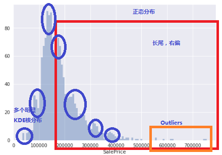
如果是老司机的话,基本上可以看出来如下几个特点:
- 基本上是正态分布(如果不是,就可以洗洗睡了,或者要重新让数据变成正态分布)
- 长尾, 尤其是右边(不是完美的正态, 看起来有清洗工作要做)
- 可能存在Outliers(异常点),特别是60万以上的房价(能处理就处理,不能就粗暴的说,我没看见。 哈哈)
- 用KDEPlot其时间能看见多个核。(在梅塞德斯奔驰比赛中,有人用聚类方法提炼出特征,也可以提高比分0.0X。由于提前引入了预测功能, 不太符合我简约的观点。 所以我的这个分享中没有专门涉及。)
接下来,火车身:
如果说combined Dataframe是火车头的输出,那么Pandas Pipe就是火车身的输入。 火车身好长,可以放很多车厢。 一节连着一节。每一节的输出是上一节的输入,直到最后。
Pandas Pipe可以作为火车身,每一个函数可以向乐高积木一样,插在一个pipe 里面。
Pipe是Pandas 里面一个Tablewise的函数(v16.2的新功能原厂说明链接)。
比较一下,下面两种方法,哪种更加简洁和易于理解?
函数方法
# f, g, and h are functions taking and returning ``DataFrames``
>>> f(g(h(df), arg1=1), arg2=2, arg3=3)
Pipe大法
>>> (df.pipe(h)
      .pipe(g, arg1=1)
      .pipe(f, arg2=2, arg3=3)
   )
尽管看起来很简洁,不过非常不起眼,貌似也没apply, map, group等明星函数受到重视。其实原厂还有一个例子,pipe就是用来做statsmodel回归特征工程的前期清洗。不过当时,我没有特别留意。 直到,Kaggle 比赛的House Price,出现瓶颈。
- local CV及pulic board成绩不稳定上升。 我刷Kaggle 出现了成绩上上下下,结果非常不稳定时。我想Pipe 把各种功能放在一起,会不会好一些?
- 调参太费时间(每次以小时计算,并且特征工程结果稍微有些改变,优化好的参数又要重新再调一遍),貌似特征工程差之毫厘,调参的参数和性能,预测的结果也会谬之千里。
-繁杂的程序,导致内存经常用光。基本上用上一会儿,就要重新启动Jupyter 的 Kernel来回收内存。 (尤其是我租的阿里云服务器只有1核1G内存+2G虚拟内存。用硬盘虚拟内存。物理内存用完后, 一个简单的回归算法也能算上几分钟时间)
这是,Pandas pipe(原厂说明链接) 重新回到了我的视野。
pipe
pipe
pipe
重要的事情说三遍。
比较早的时候,我学会了用Sklearn的pipeline和Gridsearch 一起调参,调函数,那个功能之强大是谁用谁知道。
只要备选参数设好,备选算法设好,就交给计算就可以。所以特别喜欢pipe这类自动化的东西。 可以把苦脏累的活一下子变成高大上的,可以偷懒的活。训练虽然花时间,还是有pipeline的套路可以使用。
不过在发现和利用Pandas 的pipe之前,特征工程简直就是苦脏累的活。例如:
- 大量的特征需要琢磨,
尤其是House Price 这个案例,一共有80个特征,1个目标(售价)。 为了搞明白美国的房价到底和那些有关,我还特别读了好几篇美国的房价深度分析报告。然并卵,这些特征还会互相影响。
- 绝大多数的特征都不知道琢磨后是否有价值,(单变量回归)
例如,房子外立面材料,房间的电器开关用的什么标准,多少安培等等等,Frontage大小,宗土图形状等等, 贷款是否还清了,
- 更不知道和其他特征配合后结果会如何。(多元变量回归)
街区,成交的月份,年份(中间还有07,08年经济危机),房屋大小,宗土面积互相关关联。
- 是不是有聚类的情况(非监管内机器学习方法)
前两天刚学了一个知识,用Kmeans方法可以挖掘出来新的特征。这种特征方法不是基于经验和知识,而仅仅是依赖于机器学习。
插句话,特征工程,尤其本文后面附录的的特征工程函数,大量依赖于个人的经验和知识水平,老司机和新司机的特征工程结果会差别很大。 基于机器学习的特征工程,应该是未来的一个趋势。前两个月在网上看到以为百度前搜索广告推广工程师发的文章。讲的就是百度在2010年前后的变化,之前还是比较依赖于人工的特征工程。后来特征工程太多,人工完全无法适应,他用类似的Kmeans方法作了聚类方法的特征工程(希望我没记错)。
上面说了4中特征工程的苦脏累。 我在House Price 比赛中全都碰到了。 前期还有点兴趣,后期简直是乏味。 在加上我的机器学习环境只有 1核1G内存的Centos阿里云主机。经常调试就内存用光来,或者变成用硬盘虚拟内存,慢的无法忍受。
Pandas pipe来了, 简单,有效。 可以有效地隔离,有效地连接,并且可以批量产生大量特征工程结果组合。
上面唠叨了许多Pipe的文字观点,也许读者已经有点烦了,下面再上两张积木的照片,来图示比较积木和pipe的关系。
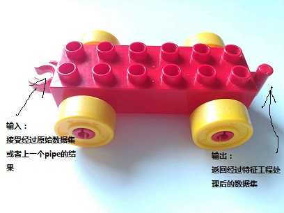 Pipe 就像乐高小火车积木中的车身,本身没有任何功能,但是有很好的输入、输出机制
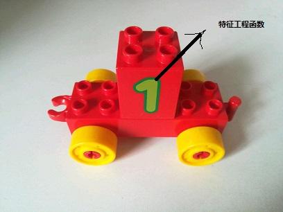 车身搭上一个积木,小火车好玩。Pipe也要装入特征工程函数,才有用
 两个或者更多车身积木连在一起,就变成长长的火车身。两个或者多个pipe(装入特征函数)就变成了特征工程管道
接下来,我们来看看,这个积木方法是否能够解决特征工程中4个问题?
- 大量的特征需要琢磨,
一个特征就来一个pipe。pipe里面放对应的特征函数。多个特征就用多个pipe.
虽然大量的特征依然需要逐一琢磨。但是pipe可能带入项目管理中WBS工作分解的思路。把多个特征分解给不同的人(不同领域有不同的专家)来做,最后用pipe链接起来。
- 绝大多数的特征都不知道琢磨后是否有价值,(单变量分析)
pipe分解了特征工作后,每一个具体的特征函数,可以深入的使用本领域的方法来设kpi和指标,在函数级别确定是否有价值,或者设定处理的量纲,过滤级别等等。
- 更不知道和其他特征配合后结果会如何。(多元变量回归)
pipe的强处就在这里。搭积木呀,简单的各种pipe连在一起就好。甚至还可以专门做一个测试成绩的pipe.在pipes的结尾放一个快速测试函数(例如:测试R2)就可以方便快速的得到这次特征工程大致效果。
注:
回归类比赛,成绩通常是两种:R2 或者是 MSE以及其变种(RMSE,AMSE等)
分类内比赛,成绩类型比较多:accuracy, precise,f1, mutual等等。
- 是不是有聚类的情况(非监管内机器学习方法)
简单,做一个聚类的特征函数,然后用一个pipe装起来就好。
下面,开始无聊的代码时间吧!
机器环境:
硬件- 阿里云最便宜一款 -1核 1GB(共享基本型 xn4,ecs.xn4.small)(
系统 , Centos 7(虚拟内存2G)
Python: 3.6, Jupyter notebook 4.3, 用Anaconda装好了常见的科学计算库。
手工装了:XGBoost(kaggle刷分利器之一) , lightbm 库(微软开源,速度比XGBoost快)。有两上面这两个库,sklearn 里面的gradientboost就没有必要用了,太慢了,score也不如这两个库好。
- 1.导入函数和Panas库
import numpy as np
import pandas as pd
from my-lib import *
#例如: eda_plot
#定义函数和pipe都放在my-lib里面(这部分没有测试过)。我用my-lib.func方式来调用这些函数
#为了文章显示美观,我在最后逐一分享函数,实际代码这些函数是方法最前面的
from datetime import datetime
import matplotlib.pyplot as plt
import seaborn as sns
%matplotlib inline

SKIPMAP = False #此外全局变量开关,用来关闭/启动自定义函数的画图。节约时间和内存
#注:特征工程阶段一般来说Pandas 和numpy就够了。 本文侧重特征工程,EDA部分跳过,不谈。
- 2.导入数据,准备combined数据集。做好火车头
train = pd.read_csv("train.csv.gz")
test = pd.read_csv("test.csv.gz")

combined = pd.concat([train,test],axis =0, ignore_index =True)
ntrain = train.shape[0]
Y_train = train["SalePrice"]
X_train = train.drop(["Id","SalePrice"],axis=1)
print("train data shape:\t ",train.shape)
print("test data shape:\t ",test.shape)
print("combined data shape:\t",combined.shape)
train data shape: (1460, 81)
test data shape: (1459, 80)
combined data shape: (2919, 81)
数据集:train 1460个,test,1459个,特征为80个,另外一个是需要预测的目标(SalePrice)
- 3. Exploring Data analysis 数据探索分析
3.1 要事第一,先看看目标数据情况(Y -SalePrice)
print(Y_train.skew()) #skew是单变量工具,用来监测数据是否有长尾,左偏或者右偏
eda_plot(cols=["SalePrice"])
#自定义函数,用来显示单变量的正太分布图和双变量(和销售价格)关系图。
文章开头已经介绍过了,销售价格是正态分布,但是长尾(high skews)且有离散点(outliers)
- 3.2 特征分析 (X), 80个,每列代表了一个特征
- 3.2.1 偏度分析 - 销售价格由偏度角度,那么就先对特征检查一下偏度。
np.abs(combined[:ntrain].skew()).sort_values(ascending = False ).head(20)
#np.abs 是绝对值函数,用来取整个向量绝对值
MiscVal 24.476794
PoolArea 14.828374
LotArea 12.207688
3SsnPorch 10.304342
LowQualFinSF 9.011341
KitchenAbvGr 4.488397
BsmtFinSF2 4.255261
ScreenPorch 4.122214
BsmtHalfBath 4.103403
EnclosedPorch 3.089872
MasVnrArea 2.669084
OpenPorchSF 2.364342
LotFrontage 2.163569
SalePrice 1.882876
BsmtFinSF1 1.685503
WoodDeckSF 1.541376
TotalBsmtSF 1.524255
MSSubClass 1.407657
1stFlrSF 1.376757
GrLivArea 1.366560
dtype: float64
看起来蛮厉害,前面20个特征偏度都超过了1.36。后期需要处理
Found:
More than 20 features(columns) showed high skews(left,right).
Next Actions:
if the skew() value > certain value, they have to been transfer by log1p to improve the accuracy
3.2.2 缺失值分析
cols_missing_value = combined.isnull().sum()/combined.shape[0]
cols_missing_value = cols_missing_value[cols_missing_value>0]
print("How many features is bad/missing value? The answer is:",cols_missing_value.shape[0])
cols_missing_value.sort_values(ascending=False).head(10).plot.barh()
How many features is bad/missing value? The answer is: 35
Out[10]:
<matplotlib.axes._subplots.AxesSubplot at 0x7f303cf5aef0>
有35个数据都有缺失值情况。 大多数机器学习算法要求不可以有缺失值。 因此,处理缺失值是 必要工作之一。
Fill the missing value is first step to in Machine learning as most of the learning estimator expect the pre-process data.
Found:
35 features were found missing values
top 6 features missed more than 50% of data. They were: PoolQC, MiscFeature, Alley, Fence, FirePlaceQu
Next Actions:
All features found missing value will be fillNA with different approaches. for example:
Basic_fillna, Just fiilna with median/mean(). In this case, we choise median as significant skew() was identified. It quick & easy.
Manual_fillna, fillna with detail data exploring manually. It will be time consuming actions & manual handled, some time depend on the people peronsal experience. To wash the data with my knowledge(maybe bias), and fillNA with
grouped mean/medain (based on location, similar group)
specific values.(0, "NA",and etc)
总结:初步EDA了解到:
1.有偏度 - 需要处理。通常是用log1p (提分关键)
2.有缺失 - 需要填充或者删除,通常用均值或者中指,或者用人工分析(人工分析是提分关键)
3.有类别变量 - 需要转换成数值 (个人感觉刷近前20%关键)
(此处没有做EDA, 直接看data_description.txt文件)
- 4.准备pipe,装载特征函数,小火车出发啦!!!
from my-lib import *
#导入一下自定义的特征函数
#例如:
#定义函数和pipe都放在my-lib里面(这部分没有测试过)。我用my-lib.func方式来调用这些函数
#为了文章显示美观,我在最后逐一分享函数,实际代码这些函数是方法最前面的
为了演示,我定义三个pipes, 每个pipes里面都有若干个特征处理函数和一个快速测试R2(越高越好,最大值是1)的函数。实际刷分时更多,加上不同的特征函数参数,做的pipes组合大概至少几十种。
为了对齐美观,用bypass函数来填充空白的地方。用一个列表,将这三个pipe放入。
现在三辆火车准备出发,都在车站等候待命。 他们分别是简单型,自定义型(部分特征转换成有序的category类型),和概念型(提炼并新增加房屋每平米单价系数)。
pipe_basic = [pipe_basic_fillna,pipe_bypass,\
              pipe_bypass,pipe_bypass,\
              pipe_bypass,pipe_bypass,\
              pipe_log_getdummies,pipe_bypass, \
              pipe_export,pipe_r2test]


pipe_ascat = [pipe_fillna_ascat,pipe_drop_cols,\
              pipe_drop4cols,pipe_outliersdrop,\
              pipe_extract,pipe_bypass,\
              pipe_log_getdummies,pipe_drop_dummycols, \
              pipe_export,pipe_r2test]

pipe_ascat_unitprice = [pipe_fillna_ascat,pipe_drop_cols,\
              pipe_drop4cols,pipe_outliersdrop,\
              pipe_extract,pipe_unitprice,\
              pipe_log_getdummies,pipe_drop_dummycols, \
              pipe_export,pipe_r2test]

pipes = [pipe_basic,pipe_ascat,pipe_ascat_unitprice ]
好了,小火车启动了,发车。
for i in range(len(pipes)):
    print("*"*10,"\n")
    pipe_output=pipes[i]
    output_name ="_".join([x.__name__[5:] for x in pipe_output if x.__name__ is not "pipe_bypass"])
    output_name = "PIPE_" +output_name
    print(output_name)
    (combined.pipe(pipe_output[0])
             .pipe(pipe_output[1])
             .pipe(pipe_output[2])
             .pipe(pipe_output[3])
             .pipe(pipe_output[4])
             .pipe(pipe_output[5])
             .pipe(pipe_output[6])
             .pipe(pipe_output[7])
             .pipe(pipe_output[8],name=output_name)
             .pipe(pipe_output[9])
             )
精简的结果如下:
PIPE_basic_fillna_log_getdummies_export_r2test
****Testing*****
R2 Scoring by lightGBM = 0.7290 PIPE_fillna_ascat_drop_cols_drop4cols_outliersdrop_extract_log_getdummies_drop_dummycols_export_r2test
*****Drop outlier based on ratio > 0.999 quantile :
****Testing*****
R2 Scoring by lightGBM = 0.7342 PIPE_fillna_ascat_drop_cols_drop4cols_outliersdrop_extract_unitprice_log_getdummies_drop_dummycols_export_r2test
*****Drop outlier based on ratio > 0.999 quantile :
****Testing*****
R2 Scoring by lightGBM = 0.7910
三个pipes的r2(默认参数,无优化调参)结果分别是
0.729, (填充均值)
0.7390,(自定义填充,和类型转换)
0.7910(增加单价的特征工程)
那么在这一步,我们可以初步看到三个特征工程的性能。并且文件已经输出到hd5格式文件。后期在训练和预测时,直接取出预处理的文件就可以。
好了,特征工程到这里就完成了。这三个小火车PIPES的R2结果不是最好,只能说尚可。都保留下来。可以进入训练,优化,调参,集成的阶段了。本文也就写完了。
注:特征工程函数代码见文章最后部分。
非常感谢你的阅读和花费的时间。
如果本文的点赞数量超过100,那么我将会完成第三步分 Sklearn的 pipeline 调参大法。
同时你会发现本文中三个小火车里面有一个已经埋下了过拟合的种子。
分享是对自己最好的投资!
======================================================
如果,你读到这里还有耐心继续往下看的话,我把几个重要的函数分享出来。
注:火车头要保护好。 Pipe里面的第一个特征函数一定要用 copy函数获得一份完整DataFrame.这样可以避免原始数据被修改,且不能重复使用的问题。
def pipe_basic_fillna(df=combined):
    local_ntrain = ntrain
    pre_combined=df.copy()

    #print("The input train dimension:\t", pre_combined[0:ntrain].shape)
    #print("The input test dimension:\t", pre_combined[ntrain:].drop("SalePrice",axis=1).shape)

    num_cols = pre_combined.drop(["Id","SalePrice"],axis=1).select_dtypes(include=[np.number]).columns
    cat_cols = pre_combined.select_dtypes(include=[np.object]).columns


    pre_combined[num_cols]= pre_combined[num_cols].fillna(pre_combined[num_cols].median())
    # Median is my favoraite fillna mode, which can eliminate the skew impact.
    pre_combined[cat_cols]= pre_combined[cat_cols].fillna("NA")
    pre_combined= pd.concat([pre_combined[["Id","SalePrice"]],pre_combined[cat_cols],pre_combined[num_cols]],axis=1)
    return pre_combined
def pipe_drop4cols(pre_combined=pipe_fillna_ascat()):
    cols_drop =['PoolQC', 'MiscFeature', 'Alley', 'Fence', 'FireplaceQu']
    # the 4 features(columns was identified earlier which missing data >50%)
    #pre_combined, ntrain = customize_fillna_extract_outliersdrop()
    #pre_combined = customize_fillna_extract_outliersdrop()
    pre_combined = pre_combined.drop(cols_drop,axis=1)

    return pre_combined
def pipe_drop_cols(pre_combined = pipe_fillna_ascat()):
    pre_combied = pre_combined.drop(['Street', 'Utilities', 'Condition2', 'RoofMatl', 'Heating'], axis = 1)

    return pre_combined
def pipe_fillna_ascat(df=combined):
    from datetime import datetime
    local_ntrain = train.shape[0]

    pre_combined=df.copy()


    #convert quality feature to category type
    #def feature group with same categories value
    cols_Subclass = ["MSSubClass"]
    cols_Zone = ["MSZoning"]
    cols_Overall =["OverallQual","OverallCond"]

    cols_Qual = ["BsmtCond","BsmtQual",\
                 "ExterQual","ExterCond",\
                 "FireplaceQu","GarageQual","GarageCond",\
                 "HeatingQC","KitchenQual",
                "PoolQC"]
    cols_BsmtFinType = ["BsmtFinType1","BsmtFinType2"]
    cols_access = ["Alley","Street"]
    cols_condition = ["Condition1","Condition2"]
    cols_fence =["Fence"]
    cols_exposure = ["BsmtExposure"]
    cols_miscfeat = ["MiscFeature"]
    cols_exter = ["Exterior1st","Exterior2nd"]
    cols_MasVnr =["MasVnrType"]
    cols_GarageType = ["GarageType"]
    cols_GarageFinish =["GarageFinish"]
    cols_Functional = ["Functional"]
    cols_Util =["Utilities"]
    cols_SaleType = ["SaleType"]
    cols_Electrical = ["Electrical"]


    #define the map of categories valus group
    cat_Subclass = ["20",#1-STORY 1946 & NEWER ALL STYLES
                    "30",#1-STORY 1945 & OLDER
                    "40",#1-STORY W/FINISHED ATTIC ALL AGES
                    "45",#1-1/2 STORY - UNFINISHED ALL AGES
                    "50",#1-1/2 STORY FINISHED ALL AGES
                    "60",#2-STORY 1946 & NEWER
                    "70",#2-STORY 1945 & OLDER
                    "75",#2-1/2 STORY ALL AGES
                    "80",#SPLIT OR MULTI-LEVEL
                    "85",#SPLIT FOYER
                    "90",#DUPLEX - ALL STYLES AND AGES
                    "120",#1-STORY PUD (Planned Unit Development) - 1946 & NEWER
                    "150",#1-1/2 STORY PUD - ALL AGES
                    "160",#2-STORY PUD - 1946 & NEWER
                    "180",#PUD - MULTILEVEL - INCL SPLIT LEV/FOYER
                    "190",#2 FAMILY CONVERSION - ALL STYLES AND AGES
                   ]
    cat_Zone = ["A",#Agriculture
                "C (all)",#Commercial #the train/test value is different than the data_description file.
                "FV",#Floating Village Residential
                "I",#Industrial
                "RH",#Residential High Density
                "RL",#Residential Low Density
                "RP",#Residential Low Density Park
                "RM",#Residential Medium Density
               ]
    cat_Overall = ["10","9","8","7","6","5","4","3","2","1"]
    cat_Qual = ["Ex","Gd","TA","Fa","Po","NA"]
    cat_BsmtFinType = ["GLQ","ALQ","BLQ","Rec","LwQ","Unf","NA"]
    cat_access = ["Grvl","Pave","NA"]
    cat_conditions= ["Artery","Feedr","Norm","RRNn","RRAn","PosN","PosA","RRNe","RRAe"]
    cat_fence = ["GdPrv",#Good Privacy
                "MnPrv",#Minimum Privacy
                "GdWo",#Good Wood
                "MnWw",#Minimum Wood/Wire
                "NA",#No Fence
                ]
    cat_exposure = ["Gd", #Good Exposure
                    "Av", #Average Exposure (split levels or foyers typically score average or above)
                    "Mn", #Mimimum Exposure
                    "No", #No Exposure
                    "NA", #No Basement
                   ]
    cat_miscfeat = ["Elev",#Elevator
                    "Gar2",#2nd Garage (if not described in garage section)
                    "Othr",#Other
                    "Shed",#Shed (over 100 SF)
                    "TenC",#Tennis Court
                    "NA",#None
                   ]
    cat_exter =["AsbShng",#Asbestos Shingles
                "AsphShn",#Asphalt Shingles
                "BrkComm",#Brick Common Brk Cmn BrkComm
                "BrkFace",#Brick Face
                "CBlock",#Cinder Block
                "CementBd",#Cement Board #CementBd was the  data_description value
                "HdBoard",#Hard Board
                "ImStucc",#Imitation Stucco
                "MetalSd",#Metal Siding
                "Other",#Other
                "Plywood",#Plywood
                "PreCast",#PreCast,#
                "Stone",#Stone
                "Stucco",#Stucco
                "VinylSd",#Vinyl Siding
                "Wd Sdng",#Wood Siding
                "WdShing",#Wood Shingles #Wd Shng WdShing
                    ]
    cat_MasVnr =["BrkCmn",#Brick Common
                "BrkFace",#Brick Face
                "CBlock",#Cinder Block
                "None",#None
                "Stone",#Stone
                ]
    cat_GarageType =["2Types",#More than one type of garage
                    "Attchd",#Attached to home
                    "Basment",#Basement Garage
                    "BuiltIn",#Built-In (Garage part of house - typically has room above garage)
                    "CarPort",#Car Port
                    "Detchd",#Detached from home
                    "NA",#No Garage
                    ]
    cat_GarageFinish =["Fin",#Finished
                        "RFn",#Rough Finished,#
                        "Unf",#Unfinished
                        "NA",#No Garage
                      ]
    cat_Functional = ["Typ",#Typical Functionality
                    "Min1",#Minor Deductions 1
                    "Min2",#Minor Deductions 2
                    "Mod",#Moderate Deductions
                    "Maj1",#Major Deductions 1
                    "Maj2",#Major Deductions 2
                    "Sev",#Severely Damaged
                    "Sal",#Salvage only
                    ]
    cat_Util =["AllPub",#All public Utilities (E,G,W,& S)
               "NoSewr",#Electricity, Gas, and Water (Septic Tank)
                "NoSeWa",#Electricity and Gas Only
                "ELO",#Electricity only,#
                ]
    cat_SaleType =["WD",#Warranty Deed - Conventional
                   "CWD",#Warranty Deed - Cash
                    "VWD",#Warranty Deed - VA Loan
                    "New",#Home just constructed and sold
                    "COD",#Court Officer Deed/Estate
                    "Con",#Contract 15% Down payment regular terms
                    "ConLw",#Contract Low Down payment and low interest
                    "ConLI",#Contract Low Interest
                    "ConLD",#Contract Low Down
                    "Oth",#Other
                    ]
    cat_Electrical = ["SBrkr",#Standard Circuit Breakers & Romex
                        "FuseA",#Fuse Box over 60 AMP and all Romex wiring (Average),#
                        "FuseF",#60 AMP Fuse Box and mostly Romex wiring (Fair)
                        "FuseP",#60 AMP Fuse Box and mostly knob & tube wiring (poor)
                        "Mix",#Mixed
                        ]


    ###########################################################################
    #define the collection of group features &categories value by diction type
    Dict_category={"Qual":[cols_Qual,cat_Qual,"NA","Ordinal"],
                   "Overall":[cols_Overall,cat_Overall,"5","Ordinal"], # It is integer already. no need overwork
                   "BsmtFinType":[cols_BsmtFinType,cat_BsmtFinType,"NA","Ordinal"],
                   "Access":[cols_access,cat_access,"NA","Ordinal"],
                    "Fence":[cols_fence,cat_fence,"NA","Ordinal"],
                   "Exposure":[cols_exposure,cat_exposure,"NA","v"],
                   "GarageFinish":[cols_GarageFinish,cat_GarageFinish,"NA","Ordinal"],
                   "Functional":[cols_Functional,cat_Functional,"Typ","Ordinal"], #fill na with lowest quality
                   "Utility":[cols_Util,cat_Util,"ELO","Ordinal"], # fillNA with lowest quality

                   "Subclass":[cols_Subclass,cat_Subclass,"NA","Nominal"],
                   "Zone":[cols_Zone,cat_Zone,"RL","Nominal"], #RL is most popular zone value. "C(all) is the study result"
                   "Cond":[cols_condition,cat_conditions,"Norm","Nominal"],
                   "MiscFeature":[cols_miscfeat,cat_miscfeat,"NA","Nominal"],
                   "Exter":[cols_exter,cat_exter,"Other","Nominal"],
                   "MasVnr":[cols_MasVnr,cat_MasVnr,"None","Nominal"],
                   "GarageType":[cols_GarageType,cat_GarageType,"NA","Nominal"],
                   "SaleType":[cols_SaleType, cat_SaleType,"WD","Nominal"],
                   "Electrical":[cols_Electrical,cat_Electrical,"SBrkr","Nominal"],
                   }


    #Change input feature type to string, especailly to below integer type
    pre_combined[cols_Overall] = pre_combined[cols_Overall].astype(str)
    pre_combined[cols_Subclass] = pre_combined[cols_Subclass].astype(str)


    #fix the raw data mistyping
    exter_map = {"Brk Cmn":"BrkComm",
                 "CmentBd":"CementBd",
                 "CemntBd":"CementBd",
                 "Wd Shng":"WdShing" }
    pre_combined[cols_exter]=pre_combined[cols_exter].replace(exter_map)

    for v in Dict_category.values():
        cols_cat = v[0]
        cat_order =v[1]
        cat_fillnavalue=v[2]
        pre_combined[cols_cat]=pre_combined[cols_cat].fillna(cat_fillnavalue)
        #if not isOrdinal:
        if v[3] =="Nominal":
            for col in cols_cat:
                pre_combined[col]=pre_combined[col].astype('category',ordered =True,categories=cat_order)
        elif v[3]=="Ordinal":
            for col in cols_cat:
                pre_combined[col]=pre_combined[col].astype('category',ordered =True,categories=cat_order).cat.codes
                pre_combined[col] = pre_combined[col].astype(np.number)


    #pre_combined[cols_Overall] = pre_combined[cols_Overall].fillna(pre_combined[cols_Overall].median())

    #Lotfrontage fill mssing value

    pre_combined["LotFrontage"] = pre_combined.groupby("Neighborhood")["LotFrontage"].transform(lambda x: x.fillna(x.median()))


    #fill missing value to Garage related features
    #Assuming no garage for thos missing value
    pre_combined["GarageCars"] =pre_combined["GarageCars"].fillna(0).astype(int)
    pre_combined["GarageArea"] =pre_combined["GarageArea"].fillna(0).astype(int)

    #fill missing value to Basement related features
    pre_combined[["BsmtFinSF1","BsmtFinSF2","BsmtUnfSF"]]= pre_combined[["BsmtFinSF1","BsmtFinSF2","BsmtUnfSF"]].fillna(0)
    pre_combined["TotalBsmtSF"]= pre_combined["BsmtFinSF1"] + pre_combined["BsmtFinSF2"]+pre_combined["BsmtUnfSF"]

    cols_Bsmt_Bath = ["BsmtHalfBath","BsmtFullBath"]
    pre_combined[cols_Bsmt_Bath] =pre_combined[cols_Bsmt_Bath].fillna(0) #assuming mean

    pre_combined["MasVnrArea"] = pre_combined["MasVnrArea"].fillna(0) #filled per study

    #solve Year related feature missing value
    #cols_time = ["YearBuilt","YearRemodAdd","GarageYrBlt","MoSold","YrSold"]
    pre_combined["GarageYrBlt"] = pre_combined["GarageYrBlt"].fillna(pre_combined["YearBuilt"]) #use building year for garage even no garage.

    return pre_combined
def pipe_outliersdrop(pre_combined=pipe_fillna_ascat(),ratio =0.001):
    # note, it could done by statsmodel as well. it will explored in future
    ratio =1-ratio
    ntrain = pre_combined["SalePrice"].notnull().sum()

    Y_train = pre_combined["SalePrice"][:ntrain]

    num_cols = pre_combined.select_dtypes(include=[np.number]).columns
    out_df = pre_combined[0:ntrain][num_cols]

    top5 = np.abs(out_df.corrwith(Y_train)).sort_values(ascending=False)[:5]

    #eda_plot(df=pre_combined[:ntrain],cols=top5.index)
    limit = out_df["GrLivArea"].quantile(ratio)

    # limit use to remove the outliers
    dropindex = out_df[out_df["GrLivArea"]>limit].index
    dropped_pre_combined =pre_combined.drop(dropindex)
    #*****************************
    dropped_Y_train = Y_train.drop(dropindex)
    #*****************************
    print("\n\n*****Drop outlier based on ratio > {0:.3f} quantile :".format(ratio))
    #print("New shape of collected data",dropped_pre_combined.shape)
    return dropped_pre_combined
def cat_col_compress(col, threshold=0.005):
    #copy the code from stackoverflow
    # removes the bind
    dummy_col=col.copy()

    # what is the ratio of a dummy in whole column
    count = pd.value_counts(dummy_col) / len(dummy_col)

    # cond whether the ratios is higher than the threshold
    mask = dummy_col.isin(count[count > threshold].index)

    # replace the ones which ratio is lower than the threshold by a special name
    dummy_col[~mask] = "dum_others"

    return dummy_col

def pipe_log_getdummies(pre_combined = pipe_fillna_ascat(),skew_ratio=0.75,cat_ratio=0):
    from scipy.stats import skew
    skew_limit =skew_ratio #I got this limit from Kaggle directly. Someone use 1 , someone use 0.75. I just use 0.75 by random and has no detail study yet
    cat_threshold = cat_ratio


    num_cols = pre_combined.select_dtypes(include=[np.number]).columns
    cat_cols = pre_combined.select_dtypes(include=[np.object]).columns

    #log transform skewed numeric features:
    skewed_Series = np.abs(pre_combined[num_cols].skew()) #compute skewness
    skewed_cols = skewed_Series[skewed_Series > skew_limit].index.values

    pre_combined[skewed_cols] = np.log1p(pre_combined[skewed_cols])
    skewed_Series = abs(pre_combined.skew()) #compute skewness
    skewed_cols = skewed_Series[skewed_Series > skew_limit].index.tolist()

    for col in cat_cols:
        pre_combined[col]=cat_col_compress(pre_combined[col],threshold=cat_threshold) # threshold set to zero as it get high core for all estimatior  except ridge based

    pre_combined= pd.get_dummies(pre_combined,drop_first=True)

    return pre_combined
def pipe_drop_dummycols(pre_combined=pipe_log_getdummies()):
    cols = ["MSSubClass_160","MSZoning_C (all)"]
    pre_combined=pre_combined.drop(cols,axis=1)

    return pre_combined
def pipe_export(pre_output,name):

    if (pre_output is None) :
        print("None input! Expect pre_combined dataframe name as parameter")
        return
    elif pre_output.drop("SalePrice",axis=1).isnull().sum().sum()>0:
        print("Dataframe still missing value! pls check again")
        return
    elif type(name) is not str:
        print("Expect preparing option name to generate output file")
        print("The out file name will be [Preparing_Output_<name>_20171029.h5] ")
        return
    else:
        from datetime import datetime
        savetime=datetime.now().strftime("%m-%d-%H_%M")
        directory_name = "./prepare/"
        filename = directory_name + name +"_"+ savetime +".h5"
        local_ntrain = pre_output.SalePrice.notnull().sum()
        pre_train = pre_output[0:local_ntrain]
        pre_test =pre_output[local_ntrain:].drop("SalePrice",axis=1)

        pre_train.to_hdf(filename,"pre_train")
        pre_test.to_hdf(filename,"pre_test")
        #print("\n***Exported*** :{0}".format(filename))
        #print("\ttrain set size :\t",local_ntrain)
        #print("\tpre_train shape:\t", pre_train.shape)
        #print("\tpre_test  shape:\t", pre_test.shape)
        return pre_output
def pipe_r2test(df):
    import statsmodels.api as sm
    import warnings
    warnings.filterwarnings('ignore')
    print("****Testing*****")
    train_df = df

    ntrain = train_df["SalePrice"].notnull().sum()
    train = train_df[:ntrain]
    X_train = train.drop(["Id","SalePrice"],axis =1)
    Y_train = train["SalePrice"]

    from lightgbm import LGBMRegressor,LGBMClassifier

    from sklearn.model_selection import cross_val_score
    LGB =LGBMRegressor()
    nCV=3
    score = cross_val_score(LGB,X_train,Y_train,cv=nCV,scoring="r2")
    print("R2 Scoring by lightGBM = {0:.4f}".format(score.mean()))


    #print(pd.concat([X_train,Y_train],axis=1).head())
    result = sm.OLS(Y_train, X_train).fit()


    result_str= str(result.summary())
    results1 = result_str.split("\n")[:10]

    for result in results1:
        print(result)
    print('*'*20)
    return df
def pipe_extract( pre_combined = pipe_fillna_ascat()):

    #extract 3 age feature(building, Garage, and remodel)
    pre_combined["BldAge"] = pre_combined["YrSold"] - pre_combined["YearBuilt"]
    pre_combined["GarageAge"] = pre_combined["YrSold"] - pre_combined["GarageYrBlt"]
    pre_combined["RemodelAge"] = pre_combined["YrSold"] - pre_combined["YearRemodAdd"]
    SoldYM_df = pd.DataFrame({"year":pre_combined.YrSold,"month":pre_combined.MoSold.astype("int").astype("object"),"day":1})
    SoldYM_df = pd.to_datetime(SoldYM_df,format='%Y%m%d',unit="D")
    pre_combined["SoldYM"]=SoldYM_df.apply(lambda x: x.toordinal())

    #extract total space features
    # three options for calculating the total Square feet. (Garage & basement has very high sknew, remove them )
    #pre_combined["TotalSQF"] = pre_combined["GarageArea"] + pre_combined['TotalBsmtSF']  +pre_combined["GrLivArea"]+pre_combined['1stFlrSF'] + pre_combined['2ndFlrSF']
    #pre_combined["TotalSQF"] = pre_combined['TotalBsmtSF'] + pre_combined['1stFlrSF'] + pre_combined['2ndFlrSF']

    pre_combined["TotalSQF"] = pre_combined['1stFlrSF'] + pre_combined['2ndFlrSF'] +pre_combined["GrLivArea"]
    return pre_combined
def pipe_drop_dummycols(pre_combined=pipe_log_getdummies()):
    cols = ["MSSubClass_160","MSZoning_C (all)"]
    pre_combined=pre_combined.drop(cols,axis=1)

    return pre_combined
好了,非常感谢你的阅读和花费的时间。 如果本文的点赞数量超过100,那么我将会完成第三步分 Sklearn的 pipeline 调参大法。
同时你会发现本文中三个小火车里面有一个已经埋下了过拟合的种子。
分享是对自己最好的投资!
相关链接:
Kaggle HousePrice : LB 0.11666(前15%), 用搭积木的方式(2.实践-特征工程部分)