神经网络于上世纪50年代提出,直到最近十年里才得以发展迅速,正改变着我们世界的方方面面。从图像分类到自然语言处理,研究人员正在对不同领域建立深层神经网络模型并取得相关的突破性成果。但是随着深度学习的进一步发展,又面临着新的瓶颈——只对成熟网络模型进行加深加宽操作。直到最近,Hinton老爷子提出了新的概念——胶囊网络(Capsule Networks),它提高了传统方法的有效性和可理解性。

本文将讲解胶囊网络受欢迎的原因以及通过实际代码来加强和巩固对该概念的理解。
为什么胶囊网络受到这么多的关注?
对于每种网络结构而言,一般用MINST手写体数据集验证其性能。对于识别数字手写体问题,即给定一个简单的灰度图,用户需要预测它所显示的数字。这是一个非结构化的数字图像识别问题,使用深度学习算法能够获得最佳性能。本文将以这个数据集测试三个深度学习模型,即:多层感知机(MLP)、卷积神经网络(CNN)以及胶囊网络(Capsule Networks)。
多层感知机(MLP)
使用Keras建立多层感知机模型,代码如下:
# define variables
input_num_units = 784
hidden_num_units = 50
output_num_units = 10

epochs = 15
batch_size = 128

# create model
model = Sequential([
 Dense(units=hidden_num_units, input_dim=input_num_units, activation='relu'),
 Dense(units=output_num_units, input_dim=hidden_num_units, activation='softmax'),
])

# compile the model with necessary attributes
model.compile(loss='categorical_crossentropy', optimizer='adam', metrics=['accuracy'])
打印模型参数概要:
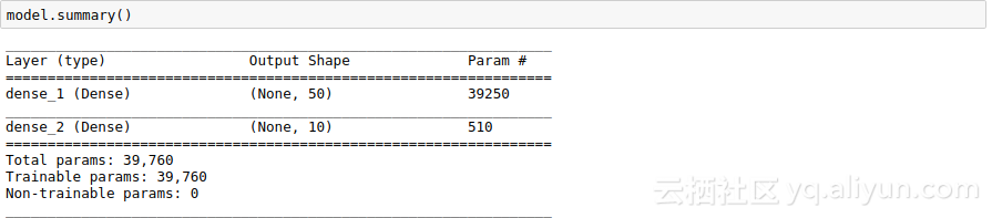
在经过15次迭代训练后,结果如下:
Epoch 14/15
34300/34300 [==============================] - 1s 41us/step - loss: 0.0597 - acc: 0.9834 - val_loss: 0.1227 - val_acc: 0.9635
Epoch 15/15
34300/34300 [==============================] - 1s 41us/step - loss: 0.0553 - acc: 0.9842 - val_loss: 0.1245 - val_acc: 0.9637
可以看到,该模型实在是简单!
卷积神经网络(CNN)
卷积神经网络在深度学习领域应用十分广泛,表现优异。下面构建卷积神经网络模型,代码如下:
# define variables
input_shape = (28, 28, 1)

hidden_num_units = 50
output_num_units = 10

batch_size = 128

model = Sequential([
 InputLayer(input_shape=input_reshape),

Convolution2D(25, 5, 5, activation='relu'),
 MaxPooling2D(pool_size=pool_size),

Convolution2D(25, 5, 5, activation='relu'),
 MaxPooling2D(pool_size=pool_size),

Convolution2D(25, 4, 4, activation='relu'),

Flatten(),

Dense(output_dim=hidden_num_units, activation='relu'),

Dense(output_dim=output_num_units, input_dim=hidden_num_units, activation='softmax'),
])

model.compile(loss='categorical_crossentropy', optimizer='adam', metrics=['accuracy'])
打印模型参数概要:
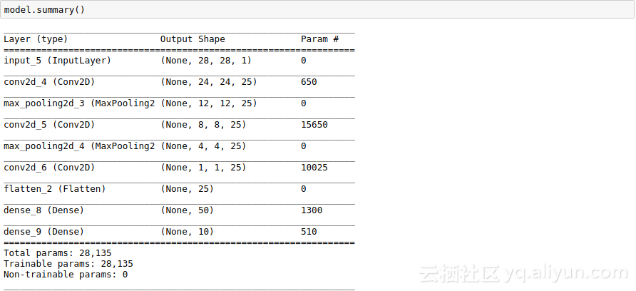
从上图可以发现,CNN比MLP模型更加复杂,下面看看其性能:
Epoch 14/15
34/34 [==============================] - 4s 108ms/step - loss: 0.1278 - acc: 0.9604 - val_loss: 0.0820 - val_acc: 0.9757
Epoch 15/15
34/34 [==============================] - 4s 110ms/step - loss: 0.1256 - acc: 0.9626 - val_loss: 0.0827 - val_acc: 0.9746
可以发现,CNN训练耗费的时间比较长,但其性能优异。
胶囊网络(Capsule Network)
胶囊网络的结构比CNN网络更加复杂,下面构建胶囊网络模型,代码如下:
def CapsNet(input_shape, n_class, routings):
   x = layers.Input(shape=input_shape)

   # Layer 1: Just a conventional Conv2D layer
   conv1 = layers.Conv2D(filters=256, kernel_size=9, strides=1, padding='valid', activation='relu', name='conv1')(x)

   # Layer 2: Conv2D layer with `squash` activation, then reshape to [None, num_capsule, dim_capsule]
   primarycaps = PrimaryCap(conv1, dim_capsule=8, n_channels=32, kernel_size=9, strides=2, padding='valid')

   # Layer 3: Capsule layer. Routing algorithm works here.
   digitcaps = CapsuleLayer(num_capsule=n_class, dim_capsule=16, routings=routings,
   name='digitcaps')(primarycaps)

   # Layer 4: This is an auxiliary layer to replace each capsule with its length. Just to match the true label's shape.
   # If using tensorflow, this will not be necessary. :)
   out_caps = Length(name='capsnet')(digitcaps)

   # Decoder network.
   y = layers.Input(shape=(n_class,))
   masked_by_y = Mask()([digitcaps, y]) # The true label is used to mask the output of capsule layer. For training
   masked = Mask()(digitcaps) # Mask using the capsule with maximal length. For prediction

   # Shared Decoder model in training and prediction
   decoder = models.Sequential(name='decoder')
   decoder.add(layers.Dense(512, activation='relu', input_dim=16*n_class))
   decoder.add(layers.Dense(1024, activation='relu'))
   decoder.add(layers.Dense(np.prod(input_shape), activation='sigmoid'))
   decoder.add(layers.Reshape(target_shape=input_shape, name='out_recon'))

   # Models for training and evaluation (prediction)
   train_model = models.Model([x, y], [out_caps, decoder(masked_by_y)])
   eval_model = models.Model(x, [out_caps, decoder(masked)])

   # manipulate model
   noise = layers.Input(shape=(n_class, 16))
   noised_digitcaps = layers.Add()([digitcaps, noise])
   masked_noised_y = Mask()([noised_digitcaps, y])
   manipulate_model = models.Model([x, y, noise], decoder(masked_noised_y))

   return train_model, eval_model, manipulate_model
打印模型参数概要:
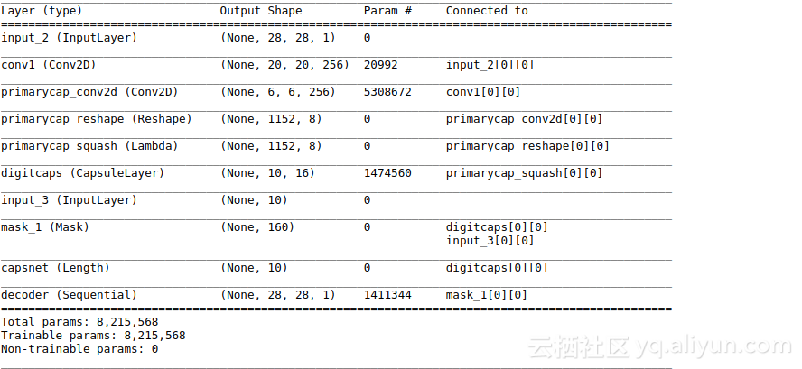
该模型耗费时间比较长,训练一段时间后,得到如下结果:
Epoch 14/15
34/34 [==============================] - 108s 3s/step - loss: 0.0445 - capsnet_loss: 0.0218 - decoder_loss: 0.0579 - capsnet_acc: 0.9846 - val_loss: 0.0364 - val_capsnet_loss: 0.0159 - val_decoder_loss: 0.0522 - val_capsnet_acc: 0.9887
Epoch 15/15
34/34 [==============================] - 107s 3s/step - loss: 0.0423 - capsnet_loss: 0.0201 - decoder_loss: 0.0567 - capsnet_acc: 0.9859 - val_loss: 0.0362 - val_capsnet_loss: 0.0162 - val_decoder_loss: 0.0510 - val_capsnet_acc: 0.9880可以发现,该网络比之前传统的网络模型效果更好,下图总结了三个实验结果:
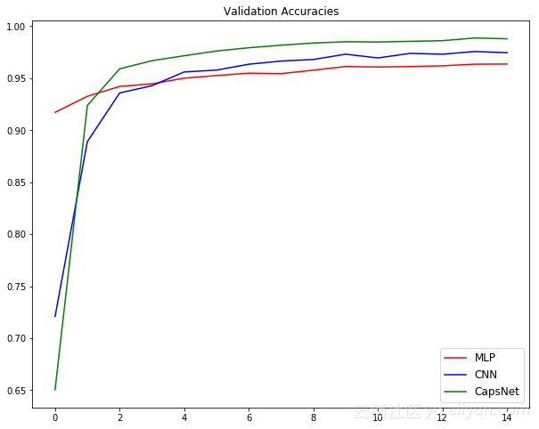
这个实验也证明了胶囊网络值得我们深入的研究和讨论。
胶囊网络背后的概念
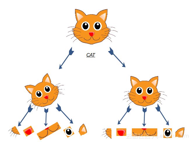
为了理解胶囊网络的概念,本文将以猫的图片为例来说明胶囊网络的潜力,首先从一个问题开始——下图中的动物是什么?

它是一只猫,你肯定猜对了吧!但是你是如何知道它是一只猫的呢?现在将这张图片进行分解:
情况1——简单图像

你是如何知道它是一只猫的呢?可能的方法是将其分解为单独的特征,如眼睛、鼻子、耳朵等。如下图所示:
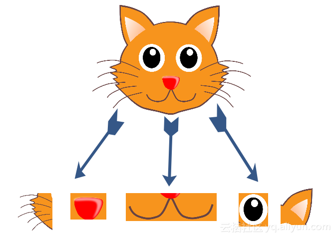
因此,本质上是把高层次的特征分解为低层次的特征。比如定义为:
P(脸) = P(鼻子) & ( 2 x P(胡须) ) & P(嘴巴) & ( 2 x P(眼睛) ) & ( 2 x P(耳朵) )
其中,P(脸) 定义为图像中猫脸的存在。通过迭代,可以定义更多的低级别特性,如形状和边缘,以简化过程。
情况2——旋转图像
将图像旋转30度,如下图所示:

如果还是按照之前定义的相同特征,那么将无法识别出它是猫。这是因为底层特征的方向发生了改变,导致先前定义的特征也将发生变化。
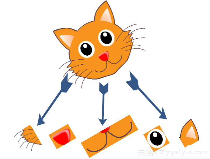
综上,猫识别器可能看起来像这样:
更具体一点,表示为:
P(脸) = ( P(鼻子) & ( 2 x P(胡须) ) & P(嘴巴) & ( 2 x P(眼睛) ) & ( 2 x P(耳朵) ) ) OR
( P(rotated_鼻子) & ( 2 x P(rotated_胡须) ) & P(rotated_嘴巴) & ( 2 x P(rotated_眼睛) ) & ( 2 x P(rotated_耳朵) ) )
情况3——翻转图像
为了增加复杂性,下面是一个完全翻转的图像:

可能想到的方法是靠蛮力搜索低级别特征所有可能的旋转,但这种方法耗时耗力。因此,研究人员提出,包含低级别特征本身的附加属性,比如旋转角度。这样不仅可以检测特征是否存在,还可以检测其旋转是否存在,如下图所示:
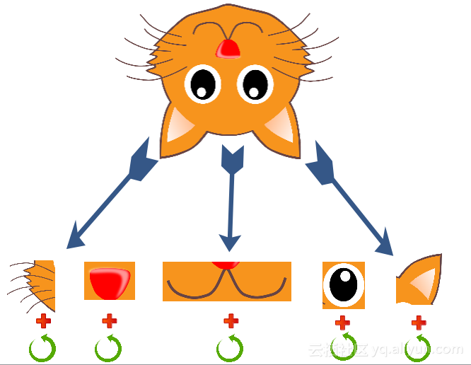
更具体一点,表示为:
P(脸) = [ P(鼻子), R(鼻子) ] & [ P(胡须_1), R(胡须_1) ] & [ P(胡须_2), R(胡须_2) ] & [ P(嘴巴), R(嘴巴) ] & …
其中,旋转特征用R()表示,这一特性也被称作旋转等价性。
从上述情况中可以看到,扩大想法之后能够捕捉更多低层次的特征,如尺度、厚度等,这将有助于我们更清楚地理解一个物体的形象。这就是胶囊网络在设计时设想的工作方式。
胶囊网络另外一个特点是动态路由,下面以猫狗分类问题讲解这个特点。
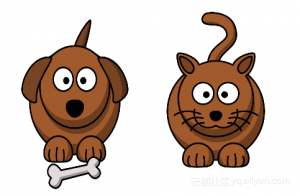
上面两只动物看起来非常相似,但存在一些差异。你可以从中发现哪只是狗吗?
正如之前所做的那样,将定义图像中的特征以找出其中的差异。
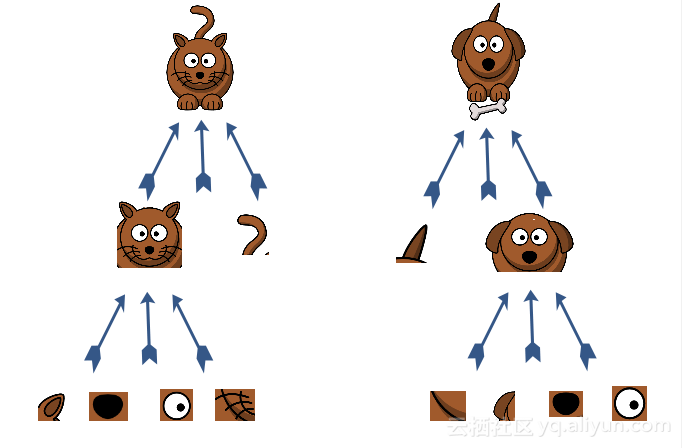
如图所示,定义非常低级的面部特征,比如眼睛、耳朵等,并将其结合以找到一个脸。之后,将面部和身体特征结合来完成相应的任务——判断它是一只猫或狗。
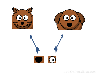
现在假设有一个新的图像,以及提取的低层特征,需要根据以上信息判断出其类别。我们从中随机选取一个特征,比如眼睛,可以只根据它来判断其类别吗?
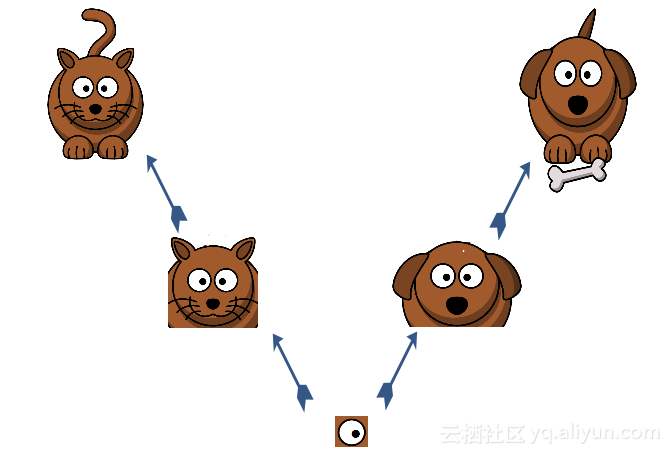
答案是否定的,因为眼睛并不是一个区分因素。下一步是分析更多的特征,比如随机挑选的下一个特征是鼻子。
只有眼睛和鼻子特征并不能够完成分类任务,下一步获取所有特征,并将其结合以判断所属类别。如下图所示,通过组合眼睛、鼻子、耳朵和胡须这四个特征就能够判断其所属类别。基于以上过程,将在每个特征级别迭代地执行这一步骤,就可以将正确的信息路由到需要分类信息的特征检测器。
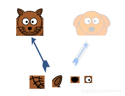
在胶囊构件中,当更高级的胶囊同意较低级的胶囊输入时,较低级的胶囊将其输入到更高级胶囊中,这就是动态路由算法的精髓。
胶囊网络相对于传统深度学习架构而言,在对数据方向和角度方面更鲁棒,甚至可以在相对较少的数据点上进行训练。胶囊网络存在的缺点是需要更多的训练时间和资源。
胶囊网络在MNIST数据集上的代码详解
首先从识别数字手写体项目下载数据集,数字手写体识别问题主要是将给定的28x28大小的图片识别出其显示的数字。在开始运行代码之前,确保安装好Keras。
下面打开Jupyter Notebook软件,输入以下代码。首先导入所需的模块:
然后进行随机初始化:
# To stop potential randomness
seed = 128
rng = np.random.RandomState(seed)
下一步设置目录路径:
root_dir = os.path.abspath('.')
data_dir = os.path.join(root_dir, 'data')下面加载数据集,数据集是“.CSV”格式。
train = pd.read_csv(os.path.join(data_dir, 'train.csv'))
test = pd.read_csv(os.path.join(data_dir, 'test.csv'))

train.head()
展示数据表示的数字:
img_name = rng.choice(train.filename)
filepath = os.path.join(data_dir, 'train', img_name)

img = imread(filepath, flatten=True)

pylab.imshow(img, cmap='gray')
pylab.axis('off')
pylab.show()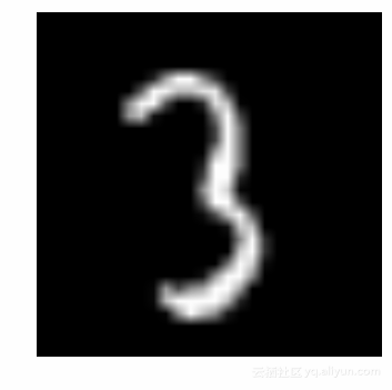
现在将所有图像保存为Numpy数组:
temp = []
for img_name in train.filename:
   image_path = os.path.join(data_dir, 'train', img_name)
   img = imread(image_path, flatten=True)
   img = img.astype('float32')
   temp.append(img)

train_x = np.stack(temp)

train_x /= 255.0
train_x = train_x.reshape(-1, 784).astype('float32')

temp = []
for img_name in test.filename:
   image_path = os.path.join(data_dir, 'test', img_name)
   img = imread(image_path, flatten=True)
   img = img.astype('float32')
   temp.append(img)

test_x = np.stack(temp)

test_x /= 255.0
test_x = test_x.reshape(-1, 784).astype('float32')

train_y = keras.utils.np_utils.to_categorical(train.label.values)
这是一个典型的机器学习问题,将数据集分成7:3。其中70%作为训练集,30%作为验证集。
split_size = int(train_x.shape[0]*0.7)

train_x, val_x = train_x[:split_size], train_x[split_size:]
train_y, val_y = train_y[:split_size], train_y[split_size:]
下面将分析三个不同深度学习模型对该数据的性能,分别是多层感知机、卷积神经网络以及胶囊网络。
1.多层感知机
定义一个三层神经网络,一个输入层、一个隐藏层以及一个输出层。输入和输出神经元的数目是固定的,输入为28x28图像,输出是代表类的10x1向量,隐层设置为50个神经元,并使用梯度下降算法训练。
# define vars
input_num_units = 784
hidden_num_units = 50
output_num_units = 10

epochs = 15
batch_size = 128

# import keras modules

from keras.models import Sequential
from keras.layers import InputLayer, Convolution2D, MaxPooling2D, Flatten, Dense

# create model
model = Sequential([
 Dense(units=hidden_num_units, input_dim=input_num_units, activation='relu'),
 Dense(units=output_num_units, input_dim=hidden_num_units, activation='softmax'),
])

# compile the model with necessary attributes
model.compile(loss='categorical_crossentropy', optimizer='adam', metrics=['accuracy'])
打印模型参数概要:
trained_model = model.fit(train_x, train_y, nb_epoch=epochs, batch_size=batch_size, validation_data=(val_x, val_y))在迭代15次之后,结果如下:
Epoch 14/15
34300/34300 [==============================] - 1s 41us/step - loss: 0.0597 - acc: 0.9834 - val_loss: 0.1227 - val_acc: 0.9635
Epoch 15/15
34300/34300 [==============================] - 1s 41us/step - loss: 0.0553 - acc: 0.9842 - val_loss: 0.1245 - val_acc: 0.9637
结果不错,但可以继续改进。
2.卷积神经网络
把图像转换成灰度图(2D),然后将其输入到CNN模型中:
# reshape data
train_x_temp = train_x.reshape(-1, 28, 28, 1)
val_x_temp = val_x.reshape(-1, 28, 28, 1)

# define vars
input_shape = (784,)
input_reshape = (28, 28, 1)


pool_size = (2, 2)

hidden_num_units = 50
output_num_units = 10

batch_size = 128
下面定义CNN模型:
model = Sequential([
 InputLayer(input_shape=input_reshape),

Convolution2D(25, 5, 5, activation='relu'),
 MaxPooling2D(pool_size=pool_size),

Convolution2D(25, 5, 5, activation='relu'),
 MaxPooling2D(pool_size=pool_size),

Convolution2D(25, 4, 4, activation='relu'),

Flatten(),

Dense(output_dim=hidden_num_units, activation='relu'),

Dense(output_dim=output_num_units, input_dim=hidden_num_units, activation='softmax'),
])

model.compile(loss='categorical_crossentropy', optimizer='adam', metrics=['accuracy'])

#trained_model_conv = model.fit(train_x_temp, train_y, nb_epoch=epochs, batch_size=batch_size, validation_data=(val_x_temp, val_y))
model.summary()
打印模型参数概要:
通过增加数据来调整进程:
# Begin: Training with data augmentation ---------------------------------------------------------------------#
def train_generator(x, y, batch_size, shift_fraction=0.1):
   train_datagen = ImageDataGenerator(width_shift_range=shift_fraction,
   height_shift_range=shift_fraction) # shift up to 2 pixel for MNIST
   generator = train_datagen.flow(x, y, batch_size=batch_size)
   while 1:
     x_batch, y_batch = generator.next()
     yield ([x_batch, y_batch])

# Training with data augmentation. If shift_fraction=0., also no augmentation.
trained_model2 = model.fit_generator(generator=train_generator(train_x_temp, train_y, 1000, 0.1),
 steps_per_epoch=int(train_y.shape[0] / 1000),
 epochs=epochs,
 validation_data=[val_x_temp, val_y])
# End: Training with data augmentation -----------------------------------------------------------------------#
CNN模型的结果:
Epoch 14/15
34/34 [==============================] - 4s 108ms/step - loss: 0.1278 - acc: 0.9604 - val_loss: 0.0820 - val_acc: 0.9757
Epoch 15/15
34/34 [==============================] - 4s 110ms/step - loss: 0.1256 - acc: 0.9626 - val_loss: 0.0827 - val_acc: 0.9746
3.胶囊网络
建立胶囊网络模型,结构如图所示:
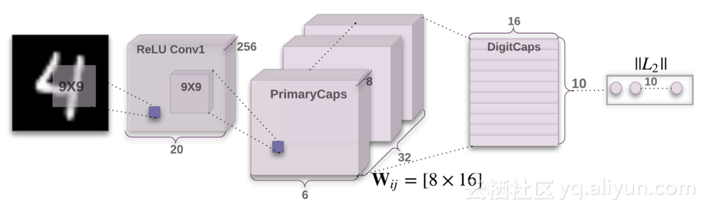
下面建立该模型,代码如下:
def CapsNet(input_shape, n_class, routings):
   """
   A Capsule Network on MNIST.
   :param input_shape: data shape, 3d, [width, height, channels]
   :param n_class: number of classes
   :param routings: number of routing iterations
   :return: Two Keras Models, the first one used for training, and the second one for evaluation.
   `eval_model` can also be used for training.
   """
   x = layers.Input(shape=input_shape)

   # Layer 1: Just a conventional Conv2D layer
   conv1 = layers.Conv2D(filters=256, kernel_size=9, strides=1, padding='valid', activation='relu', name='conv1')(x)

   # Layer 2: Conv2D layer with `squash` activation, then reshape to [None, num_capsule, dim_capsule]
   primarycaps = PrimaryCap(conv1, dim_capsule=8, n_channels=32, kernel_size=9, strides=2, padding='valid')

   # Layer 3: Capsule layer. Routing algorithm works here.
   digitcaps = CapsuleLayer(num_capsule=n_class, dim_capsule=16, routings=routings,
   name='digitcaps')(primarycaps)

   # Layer 4: This is an auxiliary layer to replace each capsule with its length. Just to match the true label's shape.
   # If using tensorflow, this will not be necessary. :)
   out_caps = Length(name='capsnet')(digitcaps)

   # Decoder network.
   y = layers.Input(shape=(n_class,))
   masked_by_y = Mask()([digitcaps, y]) # The true label is used to mask the output of capsule layer. For training
   masked = Mask()(digitcaps) # Mask using the capsule with maximal length. For prediction

   # Shared Decoder model in training and prediction
   decoder = models.Sequential(name='decoder')
   decoder.add(layers.Dense(512, activation='relu', input_dim=16*n_class))
   decoder.add(layers.Dense(1024, activation='relu'))
   decoder.add(layers.Dense(np.prod(input_shape), activation='sigmoid'))
   decoder.add(layers.Reshape(target_shape=input_shape, name='out_recon'))

   # Models for training and evaluation (prediction)
   train_model = models.Model([x, y], [out_caps, decoder(masked_by_y)])
   eval_model = models.Model(x, [out_caps, decoder(masked)])

   # manipulate model
   noise = layers.Input(shape=(n_class, 16))
   noised_digitcaps = layers.Add()([digitcaps, noise])
   masked_noised_y = Mask()([noised_digitcaps, y])
   manipulate_model = models.Model([x, y, noise], decoder(masked_noised_y))
   return train_model, eval_model, manipulate_model


def margin_loss(y_true, y_pred):
   """
   Margin loss for Eq.(4). When y_true[i, :] contains not just one `1`, this loss should work too. Not test it.
   :param y_true: [None, n_classes]
   :param y_pred: [None, num_capsule]
   :return: a scalar loss value.
   """
   L = y_true * K.square(K.maximum(0., 0.9 - y_pred)) + \
   0.5 * (1 - y_true) * K.square(K.maximum(0., y_pred - 0.1))

   return K.mean(K.sum(L, 1))
model, eval_model, manipulate_model = CapsNet(input_shape=train_x_temp.shape[1:],
 n_class=len(np.unique(np.argmax(train_y, 1))),
 routings=3)
# compile the model
model.compile(optimizer=optimizers.Adam(lr=0.001),
 loss=[margin_loss, 'mse'],
 loss_weights=[1., 0.392],
 metrics={'capsnet': 'accuracy'})

model.summary()
打印模型参数概要:
胶囊模型的结果:
Epoch 14/15
34/34 [==============================] - 108s 3s/step - loss: 0.0445 - capsnet_loss: 0.0218 - decoder_loss: 0.0579 - capsnet_acc: 0.9846 - val_loss: 0.0364 - val_capsnet_loss: 0.0159 - val_decoder_loss: 0.0522 - val_capsnet_acc: 0.9887
Epoch 15/15
34/34 [==============================] - 107s 3s/step - loss: 0.0423 - capsnet_loss: 0.0201 - decoder_loss: 0.0567 - capsnet_acc: 0.9859 - val_loss: 0.0362 - val_capsnet_loss: 0.0162 - val_decoder_loss: 0.0510 - val_capsnet_acc: 0.9880
为了便于总结分析,将以上三个实验的结构绘制出测试精度图:
plt.figure(figsize=(10, 8))
plt.plot(trained_model.history['val_acc'], 'r', trained_model2.history['val_acc'], 'b', trained_model3.history['val_capsnet_acc'], 'g')
plt.legend(('MLP', 'CNN', 'CapsNet'),
 loc='lower right', fontsize='large')
plt.title('Validation Accuracies')
plt.show()
从结果中可以看出,胶囊网络的精度优于CNN和MLP。
总结
本文对胶囊网络进行了非技术性的简要概括,分析了其两个重要属性,之后针对MNIST手写体数据集上验证多层感知机、卷积神经网络以及胶囊网络的性能。
作者信息
Faizan Shaikh,数据科学,深度学习初学者。
个人主页:https://www.linkedin.com/in/faizankshaikh
本文由阿里云云栖社区组织翻译,文章原标题《Essentials of Deep Learning: Getting to know CapsuleNets (with Python codes)》,作者:Faizan Shaikh,译者:海棠,审阅:Uncle_LLD。
文章为简译,更为详细的内容,请查看原文
