手把手教 | 深度学习库PyTorch（附代码）

介绍

每隔一段时间，就会有一个有潜力改变深度学习格局的python库诞生，PyTorch就是其中一员。

在过去的几周里，我一直沉浸在PyTorch中，我被它的易用性所吸引。在我使用过的各种深度学习库中，到目前为止PyTorch是最灵活最易用的。

在本文中，我们将以一种更实用的方式探索PyTorch, 其中包含了基础知识和案例研究。同时我们还将对比分别用numpy和PyTorch从头构建的神经网络，以查看它们在具体实现中的相似之处。

让我们开始吧！

注意：本文假定你对深度学习有基本的认知。如果想快速了解，请先阅读此文https://www.analyticsvidhya.com/blog/2016/03/introduction-deep-learning-fundamentals-neural-networks/

目录

PyTorch概览

深入技术

构建神经网络之Numpy VS. PyTorch

与其他深度学习库对比

案例研究 --- 用PyTorch解决图像识别问题

PyTorch的创作者说他们遵从指令式(imperative)的编程哲学。这就意味着我们可以立即运行计算。这一点正好符合Python的编程方法学，因为我们没必要等到代码全部写完才知道它是否能运行。我们可以轻松地运行一部分代码并实时检查它。对于我这样的神经网络调试人员而言，这真是一件幸事。

PyTorch是一个基于python的库，它旨在提供一个灵活的深度学习开发平台。

PyTorch的工作流程尽可能接近Python的科学计算库--- numpy。

你可能会问，我们为什么要用PyTorch来构建深度学习模型呢？我列举三点来回答这个问题：

易用的API：

支持Python：

动态计算图：

使用PyTorch还有其他一些好处，比如它支持多GPU，自定义数据加载器和简化的预处理器。

自从2016年1月初发布以来，许多研究人员已经将它纳入自己的工具箱，因为它易于构建新颖甚至非常复杂的图。话虽如此，PyTorch要想被大多数数据科学从业者所接受还需时日，因为它既是新生事物而且还在”建设中”。

深入技术

在深入细节之前，我们先了解一下PyTorch的工作流程。

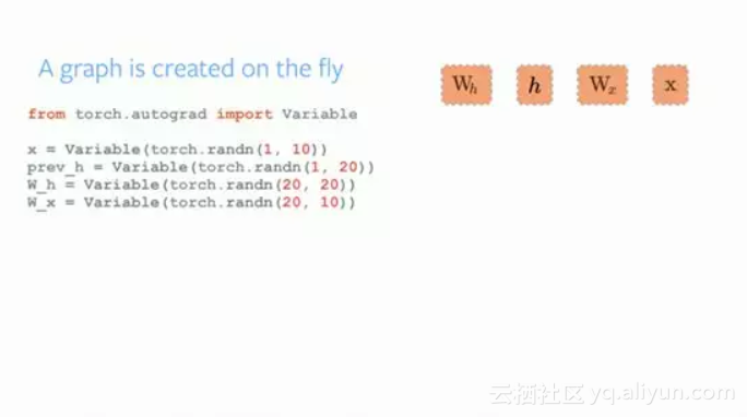
PyTorch使用了指令式编程范式。也就是说，用于构建图所需的每行代码都定义了该图的一个组件。即使在图被完全构建好之前，我们也可以在这些组件上独立地执行计算。这被称为 ”define-by-run” 方法。

Source: http://pytorch.org/about/

安装PyTorch非常简单。你可以根据你的系统，按照官方文档中提到的步骤操作。例如，下面是基于我的选项所用的命令：

conda install pytorch torchvision cuda91 -cpytorch

在我们开始使用PyTorch时，应该了解的主要元素是：

下面，我们将详细介绍每一部分。

1. PyTorch张量

张量就是多维数组。PyTorch中的张量与Numpy中的ndarrays很相似，除此之外，PyTorch中的张量还可以在GPU上使用。PyTorch支持各种类型的张量。

你可以定义一个简单的一维矩阵如下：

# import pytorch
import torch
 
# define a tensor
torch.FloatTensor([2])
2
[torch.FloatTensor of size 1]

2. 数学运算

与numpy一样，科学计算库有效地实现数学函数是非常重要的。PyTorch提供了一个类似的接口，你可以使用超过200多种数学运算。

以下是一个简单的加法操作例子：

a = torch.FloatTensor([2])
b = torch.FloatTensor([3])
 
a + b
5
[torch.FloatTensor of size 1]

这难道不像是一个典型的python方法吗？我们也可以在定义过的PyTorch张量上执行各种矩阵运算。例如，我们转置一个二维矩阵：

matrix = torch.randn(3, 3)
matrix
-1.3531 -0.5394 0.8934
 1.7457 -0.6291 -0.0484
-1.3502 -0.6439 -1.5652
[torch.FloatTensor of size 3x3]
matrix.t()
-1.3531 1.7457 -1.3502
-0.5394 -0.6291 -0.6439
 0.8934 -0.0484 -1.5652
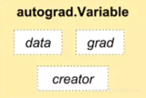
[torch.FloatTensor of size 3x3]

3. Autograd模块

PyTorch使用了一种被称为自动微分(automaticdifferentiation)的技术。也就是说，我们有一个记录器，记录了我们已经执行的操作，然后它向后重播以计算我们的梯度。这种技术在构建神经网络时特别有用，因为我们在前向传播时计算参数的微分，这可以减少每一个epoch的计算时间。

Source: http://pytorch.org/about/

from torch.autograd import Variable
 
x = Variable(train_x)
y = Variable(train_y, requires_grad=False)

4. Optim模块

Torch.optim是一个模块，它实现了用于构建神经网络的各种优化算法。大多数常用的方法已被支持，所以我们无需从头开始构建他们（除非你想！）。

以下是使用Adam优化器的一段代码：

optimizer = torch.optim.Adam(model.parameters(), lr=learning_rate)

5. nn模块

PyTorch的autograd可以很容易的定义计算图并且求梯度，但是原始的autograd对于定义复杂的神经网络可能有点过于低级。这也是nn模块可以帮忙的地方。

Nn包定义了一组模块，我们可以将其视为一个神经网络层，它可以从输入产生输出，并且可能有一些可训练的权重。

你可以把nn模块当做是PyTorch的keras!

import torch
 
# define model
model = torch.nn.Sequential(
 torch.nn.Linear(input_num_units, hidden_num_units),
 torch.nn.ReLU(),
 torch.nn.Linear(hidden_num_units, output_num_units),
)
loss_fn = torch.nn.CrossEntropyLoss()

现在你知道了PyTorch的基本组件，你可以轻松地从头构建自己的神经网络。如果你想知道具体怎么做，继续往下读。

构建神经网络之 Numpy VS. PyTorch

之前我提到PyTorch和Numpy非常相似，让我们看看为什么。在本节中，我们会看到一个简单的用于解决二元分类问题的神经网络如何实现。你可以通过https://www.analyticsvidhya.com/blog/2017/05/neural-network-from-scratch-in-python-and-r/获得深入的解释。

## Neural network in numpy
 
import numpy as np
 
#Input array
X=np.array([[1,0,1,0],[1,0,1,1],[0,1,0,1]])
 
#Output
y=np.array([[1],[1],[0]])
 
#Sigmoid Function
def sigmoid (x):
 return 1/(1 + np.exp(-x))
 
#Derivative of Sigmoid Function
def derivatives_sigmoid(x):
 return x * (1 - x)
 
#Variable initialization
epoch=5000 #Setting training iterations
lr=0.1 #Setting learning rate
inputlayer_neurons = X.shape[1] #number of features in data set
hiddenlayer_neurons = 3 #number of hidden layers neurons
output_neurons = 1 #number of neurons at output layer
 
#weight and bias initialization
wh=np.random.uniform(size=(inputlayer_neurons,hiddenlayer_neurons))
bh=np.random.uniform(size=(1,hiddenlayer_neurons))
wout=np.random.uniform(size=(hiddenlayer_neurons,output_neurons))
bout=np.random.uniform(size=(1,output_neurons))
 
for i in range(epoch):
 #Forward Propogation
 hidden_layer_input1=np.dot(X,wh)
 hidden_layer_input=hidden_layer_input1 + bh
 hiddenlayer_activations = sigmoid(hidden_layer_input)
 output_layer_input1=np.dot(hiddenlayer_activations,wout)
 output_layer_input= output_layer_input1+ bout
 output = sigmoid(output_layer_input)
 
 #Backpropagation
 E = y-output
 slope_output_layer = derivatives_sigmoid(output)
 slope_hidden_layer = derivatives_sigmoid(hiddenlayer_activations)
 d_output = E * slope_output_layer
 Error_at_hidden_layer = d_output.dot(wout.T)
 d_hiddenlayer = Error_at_hidden_layer * slope_hidden_layer
 wout += hiddenlayer_activations.T.dot(d_output) *lr
 bout += np.sum(d_output, axis=0,keepdims=True) *lr
 wh += X.T.dot(d_hiddenlayer) *lr
 bh += np.sum(d_hiddenlayer, axis=0,keepdims=True) *lr
 
print('actual :\n', y, '\n')
print('predicted :\n', output)

现在，尝试发现PyTorch超级简单的实现与之前的差异（下面代码中差异部分用粗体字表示）。

## neural network in pytorch
import torch
 
#Input array
X = torch.Tensor([[1,0,1,0],[1,0,1,1],[0,1,0,1]])
 
#Output
y = torch.Tensor([[1],[1],[0]])
 
#Sigmoid Function
def sigmoid (x):
 return 1/(1 + torch.exp(-x))
 
#Derivative of Sigmoid Function
def derivatives_sigmoid(x):
 return x * (1 - x)
 
#Variable initialization
epoch=5000 #Setting training iterations
lr=0.1 #Setting learning rate
inputlayer_neurons = X.shape[1] #number of features in data set
hiddenlayer_neurons = 3 #number of hidden layers neurons
output_neurons = 1 #number of neurons at output layer
 
#weight and bias initialization
wh=torch.randn(inputlayer_neurons, hiddenlayer_neurons).type(torch.FloatTensor)
bh=torch.randn(1, hiddenlayer_neurons).type(torch.FloatTensor)
wout=torch.randn(hiddenlayer_neurons, output_neurons)
bout=torch.randn(1, output_neurons)
 
for i in range(epoch):
 
 #Forward Propogation
 hidden_layer_input1 = torch.mm(X, wh)
 hidden_layer_input = hidden_layer_input1 + bh
 hidden_layer_activations = sigmoid(hidden_layer_input)
 output_layer_input1 = torch.mm(hidden_layer_activations, wout)
 output_layer_input = output_layer_input1 + bout
 output = sigmoid(output_layer_input1)
 
 #Backpropagation
 E = y-output
 slope_output_layer = derivatives_sigmoid(output)
 slope_hidden_layer = derivatives_sigmoid(hidden_layer_activations)
 d_output = E * slope_output_layer
 Error_at_hidden_layer = torch.mm(d_output, wout.t())
 d_hiddenlayer = Error_at_hidden_layer * slope_hidden_layer
 wout += torch.mm(hidden_layer_activations.t(), d_output) *lr
 bout += d_output.sum() *lr
 wh += torch.mm(X.t(), d_hiddenlayer) *lr
 bh += d_output.sum() *lr
print('actual :\n', y, '\n')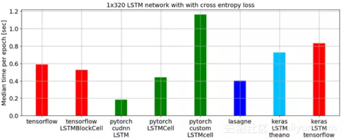
print('predicted :\n', output)

与其他深度学习库对比

在一个基准测试脚本中，通过比较最低的epoch中位数时间，PyTorch在训练一个Long Short Term Memory(LSTM)网络方面胜过了所有其他主要的深度学习库，参加下图：

用于数据加载的APIs在PyTorch中设计良好。接口在数据集，采样器和数据加载器中指定。

在比较TensorFlow中的数据加载工具(readers, queues等等)时，我发现PyTorch的数据加载模块非常易于使用。另外，PyTorch在我们尝试构建神经网络时是无缝衔接的，所以我们不必像keras那样依赖第三方高级库（keras依赖tensorflow或theano）。

另一方面，我不推荐使用PyTorch进行部署。 PyTorch尚处于发展中。正如PyTorch开发人员所说：“我们看到的是用户首先创建一个PyTorch模型，当他们准备将模型部署到生产环境时，他们只需将其转换成Caffe 2模型，然后将其发布到移动平台或其他平台。“

案例研究：用PyTorch解决图像识别问题

为了熟悉PyTorch，我们将解决Analytics Vidhya的深度学习实践问题 - 识别数字。我们来看看我们的问题陈述：

我们的问题是一个图像识别问题，从一个给定的28×28像素的图像中识别数字。我们有一部分图像用于训练，其余部分用于测试我们的模型。

首先，下载训练和测试文件。该数据集包含所有图像的压缩文件，并且train.csv和test.csv都具有相应训练和测试图像的名称。数据集中不提供任何其他特征，只是以'.png'格式提供原始图像。

让我们开始吧：

步骤0：准备

1. 导入所有必要的库：

# import modules
%pylab inline
import os
import numpy as np
import pandas as pd
from scipy.misc import imread
from sklearn.metrics import accuracy_score

2. 设置种子值，以便我们可以控制模型的随机性

# To stop potential randomness
seed = 128
rng = np.random.RandomState(seed)

3. 第一步是设置目录路径，以便安全保存！

root_dir = os.path.abspath('.')
data_dir = os.path.join(root_dir, 'data')
 
# check for existence
os.path.exists(root_dir), os.path.exists(data_dir)

步骤1：数据加载和预处理

1. 现在我们来读取数据集。他们是.csv格式，并且具有相应标签的文件名。

# load dataset
train = pd.read_csv(os.path.join(data_dir, 'Train', 'train.csv'))
test = pd.read_csv(os.path.join(data_dir, 'Test.csv'))
 
sample_submission = pd.read_csv(os.path.join(data_dir, 'Sample_Submission.csv'))
 
train.head()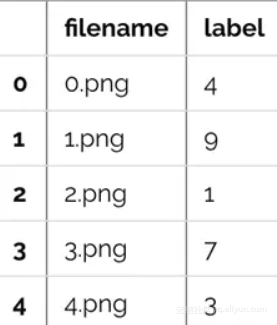

2. 我们看一下数据是什么样子，读取图片并显示。

# print an image
img_name = rng.choice(train.filename)
filepath = os.path.join(data_dir, 'Train', 'Images', 'train', img_name)
 
img = imread(filepath, flatten=True)
 
pylab.imshow(img, cmap='gray')
pylab.axis('off')
pylab.show()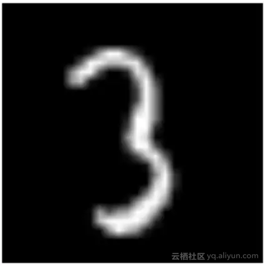

3. 为了便于数据操作，我们将所有图片存储为numpy数组。

# load images to create train and test set
temp = []
for img_name in train.filename:
 image_path = os.path.join(data_dir, 'Train', 'Images', 'train', img_name)
 img = imread(image_path, flatten=True)
 img = img.astype('float32')
 temp.append(img)
train_x = np.stack(temp)
 
train_x /= 255.0
train_x = train_x.reshape(-1, 784).astype('float32')
 
temp = []
for img_name in test.filename:
 image_path = os.path.join(data_dir, 'Train', 'Images', 'test', img_name)
 img = imread(image_path, flatten=True)
 img = img.astype('float32')
 temp.append(img)
test_x = np.stack(temp)
 
test_x /= 255.0
test_x = test_x.reshape(-1, 784).astype('float32')
 
train_y = train.label.values

4. 由于这是一个典型的ML问题，为了测试我们模型的正确功能，我们创建了一个验证集(validation set)。我们以70:30的比例来划分训练集和验证集。

# create validation set
split_size = int(train_x.shape[0]*0.7)
 
train_x, val_x = train_x[:split_size], train_x[split_size:]
train_y, val_y = train_y[:split_size], train_y[split_size:]

步骤2：构建模型

5. 现在来到了主要部分，即定义我们的神经网络架构。我们定义了一个3层神经网络即输入，隐藏和输出层。输入和输出层中的神经元数量是固定的，因为输入是我们的28×28图像，并且输出是代表类别的10×1向量。我们在隐藏层中使用50个神经元。在这里，我们使用Adam作为优化算法，它是梯度下降算法的有效变种。

import torch
from torch.autograd import Variable
# number of neurons in each layer
input_num_units = 28*28
hidden_num_units = 500
output_num_units = 10
 
# set remaining variables
epochs = 5
batch_size = 128
learning_rate = 0.001

6. 训练模型的时间到了

# define model
model = torch.nn.Sequential(
 torch.nn.Linear(input_num_units, hidden_num_units),
 torch.nn.ReLU(),
 torch.nn.Linear(hidden_num_units, output_num_units),
)
loss_fn = torch.nn.CrossEntropyLoss()
 
# define optimization algorithm
optimizer = torch.optim.Adam(model.parameters(), lr=learning_rate)
## helper functions
# preprocess a batch of dataset
def preproc(unclean_batch_x):
 """Convert values to range 0-1"""
 temp_batch = unclean_batch_x / unclean_batch_x.max()
 return temp_batch
 
# create a batch
def batch_creator(batch_size):
 dataset_name = 'train'
 dataset_length = train_x.shape[0]
 
 batch_mask = rng.choice(dataset_length, batch_size)
 
 batch_x = eval(dataset_name + '_x')[batch_mask]
 batch_x = preproc(batch_x)
 
 if dataset_name == 'train':
 batch_y = eval(dataset_name).ix[batch_mask, 'label'].values
 
 return batch_x, batch_y
# train network
total_batch = int(train.shape[0]/batch_size)
 
for epoch in range(epochs):
 avg_cost = 0
 for i in range(total_batch):
 # create batch
 batch_x, batch_y = batch_creator(batch_size)
 
 # pass that batch for training
 x, y = Variable(torch.from_numpy(batch_x)), Variable(torch.from_numpy(batch_y), requires_grad=False)
 pred = model(x)
 
 # get loss
 loss = loss_fn(pred, y)
 
 # perform backpropagation
 loss.backward()
 optimizer.step()
 avg_cost += loss.data[0]/total_batch
 
 print(epoch, avg_cost)
# get training accuracy
x, y = Variable(torch.from_numpy(preproc(train_x))), Variable(torch.from_numpy(train_y), requires_grad=False)
pred = model(x)
 
final_pred = np.argmax(pred.data.numpy(), axis=1)
 
accuracy_score(train_y, final_pred)
# get validation accuracy
x, y = Variable(torch.from_numpy(preproc(val_x))), Variable(torch.from_numpy(val_y), requires_grad=False)
pred = model(x)
final_pred = np.argmax(pred.data.numpy(), axis=1)
 
accuracy_score(val_y, final_pred)

训练得分是：

0.8779008746355685

而验证得分是：

0.867482993197279

这是一个很令人印象深刻的分数，尤其是我们只是在5个epochs上训练了一个非常简单的神经网络。

结语

我希望这篇文章能让你看到PyTorch如何改变构建深度学习模型的观点。在这篇文章中，我们只是浅尝辄止。为了深入研究，你可以阅读PyTorch官方页面上的文档和教程。