1. Introduction to Automatic Speech Recognition
1.1. What is automatic speech recognition
Research in ASR (Automatic Speech Recognition) aims to enable computers to "understand" human speech and convert it into text. ASR is the next frontier in intelligent human-machine interaction and also a precondition for perfecting machine translation and natural language understanding. Research into ASR can be traced back to the 1950s in its initial isolated word speech recognition system. Since then, with persistent efforts of numerous scholars, ASR has made significant progress and can now power large-vocabulary continuous speech recognition systems.
Especially in the emerging era of big data and application of deep neural networks, ASR systems have achieved notable performance improvements. ASR technology has also been gradually gaining practical use, becoming more product-oriented. Smart speech recognition software and applications based on ASR are increasingly entering our daily lives, in form of voice input methods, intelligent voice assistants, and interactive voice recognition systems for vehicles.
1.2. Framework of an ASR System
The purpose of ASR is to map input waveform sequences to their corresponding word or character sequences. Therefore, implementing ASR can be considered a channel decoding or pattern classification problem. Currently, statistical modeling is a core ASR method, in which, for a given speech waveform sequence O, we can use a "maximum a posteriori" (MAP) estimator, based on the mode of a posterior Bayesian distribution, to estimate the most likely output sequence W*, with the formula shown in Figure 1.
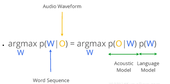
Figure 1. Mathematical formula representation of ASR
P(O|W) is the probability of generating the correct observation sequence, i.e. corresponding to the acoustic model (AM) of the ASR system, conditional on W. Likelihood P(W) is the 'a priori probability' of the exact sequence W occurring. It is called the language model (LM).
Figure 2 shows the structure diagram of a marked ASR system, which mainly comprises a frontend processing module, acoustic model, language model, and decoder. The decoding process is primarily to use the trained acoustic model and language model to obtain the optimal output sequence.
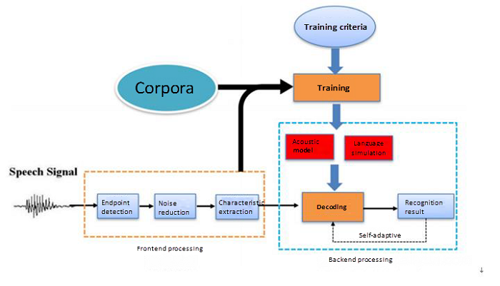
Figure 2. Structure diagram of an ASR system
1.3. Acoustic Model
An acoustic model's task is to compute the P(O|W), i.e. the probability of generating a speech waveform for the mode. An acoustic model, as an important part of the ASR system, accounts for a large part of the computational overhead and also determines the system's performance. GMM-HMM-based acoustic models are widely used in traditional speech recognition systems.
In this model, GMM is used to model the distribution of the acoustic characteristics of speech and HMM is used to model the time sequence of speech signals. Since the rise of deep learning in 2006, deep neural networks (DNNs) have been applied in speech acoustic models. In 2009, Hinton and his students used feedforward fully-connected deep neural networks in speech recognition acoustic modeling[1].
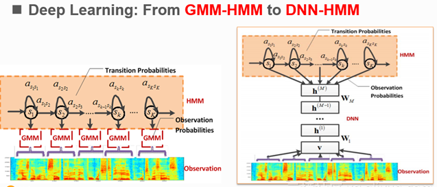
Figure 3. Comparison of GMM-HMM and DNN-HMM
Compared to traditional GMM-HMM acoustic models, DNN-HMM-based acoustic models perform better in terms of TIMIT database. When compared with GMM, DNN is advantageous in the following ways:
- De-distribution hypothesis is not required for characteristic distribution when DNN models the posterior probability of the acoustic characteristics of speech.
- GMM requires de-correlation processing for input characteristics, but DNN is capable of using various forms of input characteristics.
- GMM can only use single-frame speech as inputs, but DNN is capable of capturing valid context information by means of splicing adjoining frames.
In 2011, DengLi et al. put forward a CD-DNN-HMM-based[2] acoustic model and made success in the large vocabulary continuous speech recognition tasks, and when compared with traditional GMM-HMM systems, this system improved the performance by over 20%. DNN-HMM-based speech acoustic model started replacing GMM-HMM-based model as the mainstream model. Thereafter, many researchers have engaged in the research of speech acoustic modeling with DNNs, and ASR has gained a breakthrough progress.
2. Introduction to Papers at Interspeech 2017
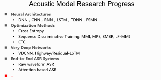
Great progress has been made in speech recognition acoustic modeling with DNNs in recent years, and with the benefits of different network structures and optimization strategies, the performance of acoustic models has been significantly improved. The following describes the latest research items of two acoustic models related to this Interspeech session: Very deep networks and End-to-end ASR systems.
2.1. Very Deep Networks for Acoustic Modeling
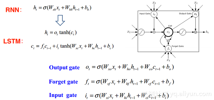
A long short-term memory (LSTM) network is a kind of recurrent neural network (RNN) structure extensively used in acoustic modeling. In comparison with general RNNs, the elaborately designed gate structure of LSTM can be used to control data storage, input, and output. At the same time, LSTM avoids the vanishing gradient problem of general RNNs to some extent, thereby enabling LSTM to effectively model the long range dependence of time sequence signals. LSTM, as an acoustic model, generally contains 3-5layers. Construction of deeper networks by stacking more LSTM layers may reduce the performance of the model due to degradation problem[3], instead of improving performance.
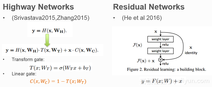
On how to optimize very deep networks, there are two kinds of structures proposed recently: Highway Network[4] and ResNet[3]. Both structures present better gradient transfer in the network training process and thus avoid the vanishing gradient problem due to deep networks by adding a linear component to the nonlinear transformation output. The difference is that a Highway Network uses "gate" to control the proportion of the linear and nonlinear components in the output, while a ResNet uses a method that directly adds a linear component. Experiments show that both can optimize the training of very deep networks. Residual Networks can obtain great successes in image classification tasks.
Both Highway Network and ResNet were tested in image classification tasks at the very beginning and convolutional neural networks (CNNs) were used. However, the importance of speech signal timing modeling makes LSTM the most popular model. In general, LSTM used in acoustic models contains 3-5 layers.
Some researchers have further optimized the structure of LSTM based on Highway Networks and ResNet, and put forward Redisual LSTM[5], Highway LSTM[6], and Recurrent Highway Networks (RHNs)[7] for speech acoustic modeling. The following section describes the corresponding network structures and experimental results by referring to the papers.
Paper 1. Residual LSTM: Design of a Deep Recurrent Architecture for Distant Speech Recognition
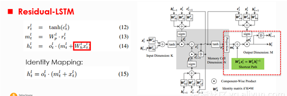
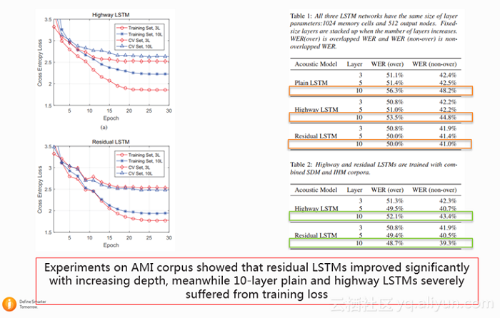
The Residual LSTM, created by adding a skip connection between general LSTM output layers, is expressed by the formula in the red box as shown in the figure above. In this way, the underlying output can be directly added to a higher layer. If the number of nodes is the same for lower and higher output layers, it is possible to further use the mapping unit in the same way as that of ResNet. The experiment result obtained by the lab from verification of a 100-hour AMI meeting database is as below:
Paper 2. Highway LSTM and Recurrent Highway Networks for Speech Recognition


The Highway LSTM, created by establishing a linear connection between cells on adjoining LSTM layers and by means of a linear transformation, adds the expression in the underlying cell to the cell in a higher layer. Meanwhile, linear transformation is controlled by a gate whose value is a function of the input of the current layer, expression in the cell of the current layer, and output at the previous moment in the cell of the next layer. This paper further puts forward another deep network structure used for acoustic modeling, which is known as Recurrent Highway Network (RHN).The hidden layer of an RHN is composed of the Recurrent Highway Layer as shown in the figure above.
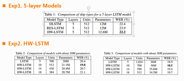
This paper was tested in a 12500-hour Google Voice Search task. The experiment firstly compared the performance of LSTM, Residual LSTM, and Highway LSTM on the task. From the experiment result of example 1 shown in the figure above, it can be seen that under comparable configurations, Highway LSTM (HW-LSTM) has better performance than Residual LSTM. In example 2, network sizes (20M and 30M) were compared, and in terms of the relationship between the performance of HW-LSTM and number of hidden layers, the result showed that Highway was capable of training a 10-layer network, and had better performance when compared to a 5-layer network. However, further increase of number of hidden layers for the network would result in reduction in the performance.
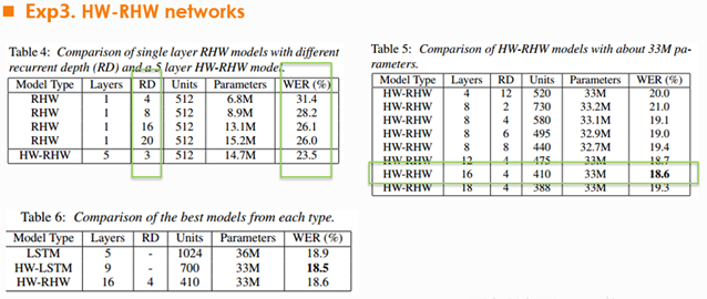
Example 3 compared the performance of Highway-Recurrent Highway Networks (HW-RHW) with different configurations on the task. The use of RHL layer allowed for successful training of very deep network. Finally, deep HW-LSTM and HW-RHW could achieve about the same performance, and work better when compared to the baseline LSTM.
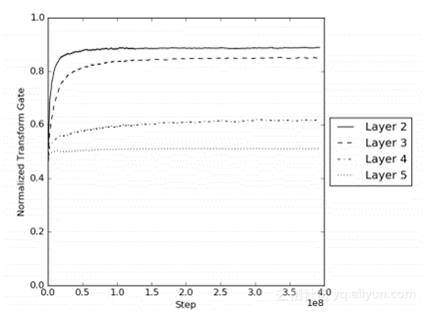
By comparing the experiment results of those two papers, we can find that, on two different task sets, the performance comparison of Highway LSTM and Residual LSTM shows opposite conclusions. This relates to the task set used in the experiment. The HW-LSTM controls the non-linear transformation and linear transformation components in the network via a gate. In general, more difficult tasks will involve more non-linear transformation models, thereby requiring stronger modeling capability. Therefore, according to the paper about Google, the HW-LSTM is advantageous on the 12500-hour task when compared to the Residual LSTM. This can be further analyzed by observing the transform gate value of each layer of HW-LSTM. The figure above shows that the transform gate value increases as the training progresses, indicating that the network tends to select the non-linear transformation component.
2.2. End-to-End ASR System
Currently, most ASR systems use a hybrid system with NN-HMM. This requires training an acoustic model and a language model and then proceeding to decoding with the aid of a dictionary. Studying end-to-end speech recognition systems with the expectation to eliminate HMM and obtain the recognized word sequence from acoustic characteristic inputs, is one of the latest research topics. Representatives are (Connectionist Temporal Classification (CTC) models and Attention-based Encoder-Decoder models.
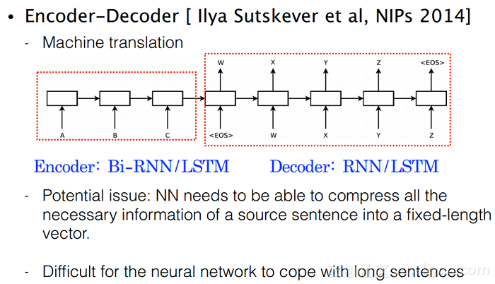
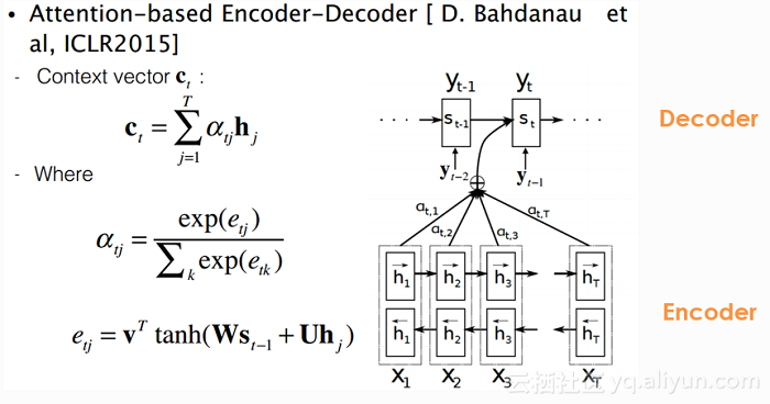
Encoder-Decoder was initially used in the machine translation field[8]: it works by encoding sequence information via the encoder to obtain a vector expression, which is then used as an input for the decoder. Decoder is a prediction model that uses the output history and information obtained by the encoder to predict an output. However, the Encoder-Decoder framework is not perfectly suitable for translating long sentences due to the problem of forgetting. An improved model was created by introducing the Attention mechanism. This mechanism uses some expressions in the network to detect certain inputs related to the current prediction outputs from the Encoder. The higher the affinity, the higher the value of the Attention vector. In this way, the Decoder is capable of obtaining an additional vector helpful in current prediction output, thus avoiding the problem of forgetting long sequences. End-to-end speech recognition can also be seen as a sequence-to-sequence translation where the input is acoustic characteristic and the output is a text sequence. As a result, the Attention-based Encoder-Decoder framework was soon applied in speech recognition. However, this framework has a problem that the Encoder must accept the whole sequence before the Decoder can generate outputs, which is unacceptable for speech recognition. For this purpose, the research at Interspeech 2017 put forward the Gaussian prediction based attention method to solve this problem. The paper is as below:
Paper 3. Gaussian Prediction Based Attention for Online End-to-End Speech Recognition
This paper has two main contributions:
1) Gaussian prediction based attention is put forward to solve the delay problem of general attention models;
2) DCNN is recommended as the Encoder and thus higher performance can be gained when compared to GRU
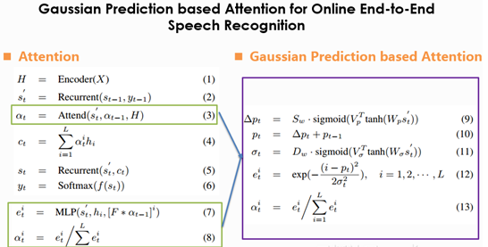
The formula expression of Gaussian prediction based attention is shown in the figure above, and the core idea is to assume the coefficient of Attention to follow the Gaussian distribution, which is acceptable in speech recognition. For a speech recognition task, both the central and peripheral frames most related to the outputs contribute to the prediction outputs, but contribution reduces as the distance increases. For this reason, unlike the traditional Attention, Gaussian prediction based attention, instead of computing the coefficient of Attention at every moment, predicts mean and variance of the Gaussian distribution. By taking into account the monotonicity of speech signal sequence, the central frame of Attention predicted in the next moment should be far back than the previous moment. Based on this, this paper used the relative prediction mode of formulas 9 and 10 to predict a positive offset rather than mean of Gaussian distribution. The mean of Gaussian distribution at the very moment is equal to the mean predicted in the previous moment plus a positive offset. At the same time, to ensure timeliness, the formula below was used for truncation:

The experiment was carried out in a 3-hour TIMIT database and the result is as below:

3. Conclusion
We hope that this article was successful in imparting knowledge about acoustic models, while also presenting latest research topics of ASR systems.
References:
[1] Mohamed A, Dahl G, Hinton G. Deep belief networks for phone recognition[C]//Nips workshop on deep learning for speech recognition and related applications. 2009, 1(9): 39.
[2] Dahl G E, Yu D, Deng L, et al. Context-dependent pre-trained deep neural networks for large-vocabulary speech recognition[J]. IEEE Transactions on audio, speech, and language processing, 2012, 20(1): 30-42.
[3] He K, Zhang X, Ren S, et al. Deep residual learning for image recognition[C]//Proceedings of the IEEE conference on computer vision and pattern recognition. 2016: 770-778.
[4] Srivastava R K, Greff K, Schmidhuber J. Highway networks[J]. arXiv preprint arXiv:1505.00387, 2015.
[5] Kim J, El-Khamy M, Lee J. Residual LSTM: Design of a Deep Recurrent Architecture for Distant Speech Recognition[J]. arXiv preprint arXiv:1701.03360, 2017.
[6] Zhang Y, Chen G, Yu D, et al. Highway long short-term memory rnns for distant speech recognition[C]//Acoustics, Speech and Signal Processing (ICASSP), 2016 IEEE International Conference on. IEEE, 2016: 5755-5759.
[7] Pundak G, Sainath T N. Highway LSTM and Recurrent Highway Networks for Speech Recognition[J]. Proc. Interspeech 2017, 2017: 1303-1307.
[8] Cho K, Van Merriënboer B, Bahdanau D, et al. On the properties of neural machine translation: Encoder-decoder approaches[J]. arXiv preprint arXiv:1409.1259, 2014.
[9] Bahdanau D, Cho K, Bengio Y. Neural machine translation by jointly learning to align and translate[J]. arXiv preprint arXiv:1409.0473, 2014.
[10] Hou J, Zhang S, Dai L. Gaussian Prediction based Attention for Online End-to-End Speech Recognition[J]. Proc. Interspeech 2017, 2017: 3692-3696.
